【菜菜的sklearn课堂笔记】聚类算法Kmeans-基于轮廓系数来选择n_clusters

视频作者：菜菜TsaiTsai
链接：【技术干货】菜菜的机器学习sklearn【全85集】Python进阶_哔哩哔哩_bilibili

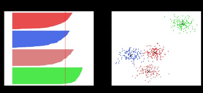
我们通常会绘制轮廓系数分布图和聚类后的数据分布图来选择我们的最佳n_clusters

from sklearn.metrics import silhouette_samples,silhouette_score
from sklearn.datasets import make_blobs
from sklearn.cluster import KMeans
import matplotlib.pyplot as plt
import matplotlib.cm as cm # colormap
import numpy as np
import pandas as pd

X,y = make_blobs(n_samples=500,n_features=2,centers=4,random_state=1)

fig,(ax1,ax2) = plt.subplots(1,2)
fig.set_size_inches(18,7) 

这里18*7是给两个子图一起用的，因此一个是$9\ast 7$

一般有关通过循环得到分数来评价模型优劣的，我们都先写其中一次的代码，然后再写循环的。在写其中一次的时候，把有关循环次数的变量都用命名的变量代替，而不是写数字，例如下面我们会用n_clusters = 4，来代替代码中的4
这里我们先写一次的代码，假设我们让它分4类

cluster = KMeans(n_clusters=n_clusters,random_state=10).fit(X)
cluster_labels = cluster.labels_
silhouette_avg = silhouette_score(X,cluster_labels)
sample_silhouette_values = silhouette_samples(X,cluster_labels)

fig,(ax1,ax2) = plt.subplots(1,2)
fig.set_size_inches(18,7)

ax1我们是为了画不同类每个样本的轮廓系数，这里我们使用填图
X.shape[0]要加上(n_clusters + 1) * 10，是为了让不同类之间以及类和轴之间有10的距离

ax1.set_xlim([-0.1,1])
ax1.set_ylim([0,X.shape[0] + (n_clusters + 1) * 10])

y_lower = 10 # 别贴着x轴画图
for i in range(n_clusters):
    ith_cluster_silhouette_values = sample_silhouette_values[cluster_labels == i]
    # array的切片之间传递的是值，而不是对象，因此修改ith_cluster_silhouette_values，不会影响sample_silhouette_values
    # 实在不安心可以.copy()
    ith_cluster_silhouette_values.sort() # .sort()排序是直接排序，没有返回值
    
    size_cluster_i = ith_cluster_silhouette_values.shape[0] # 这一簇样本的数量
    y_upper = y_lower + size_cluster_i
    
    color = cm.nipy_spectral(np.random.RandomState(i+3).random(1))
    # nipy_spectral传入一个浮点数，返回一个颜色。也可以传入浮点array
    # 这里+3没有其他目的，只是因为恰巧前四个都是绿的
    
    ax1.fill_betweenx(np.arange(y_lower,y_upper,1) # 倾向于理解是折线图的填充
                    ,ith_cluster_silhouette_values
                    ,0
                    ,facecolor=color
                    ,alpha=0.7)
    # 向x轴填充用fill_between，向y轴填充用fill_betweenx
    
    y_lower = y_upper + 10
    
    ax2.scatter(X[cluster_labels == i,0],X[cluster_labels == i,1]
               ,marker='o'
               ,s=8
               ,c=color) # 颜色和ax1的统一

ax1.text(-0.05
		 ,y_lower + 0.5 * size_cluster_i
		 ,str(i))
ax1.set_title("The silhouette plot for the various clusters.")
ax1.set_xlabel("The silhouette coefficient values")
ax1.set_ylabel("Cluster label")
ax1.axvline(x=silhouette_avg,color='red',linestyle='--')
# axvline添加一条垂直于x轴的线
ax1.set_yticks([])
ax1.set_xticks([-0.1,0,0.2,0.4,0.6,0.8,1])

centers = cluster.cluster_centers_
ax2.scatter(centers[:,0],centers[:,1],marker='x',c='k',s=200)
ax2.set_title("The visualization of the clustered data.")
ax2.set_xlabel("Feature space for the 1st feature")
ax2.set_ylabel("Feature space for the 2nd feature")
plt.suptitle(("Silhouette analysis for KMeans clustering on sample data with n_clusters = %d" % n_clusters)
             ,fontsize=14, fontweight='bold')
plt.show()

fill_betweenx(
['y', 'x1', 'x2=0', 'where=None', 'step=None', 'interpolate=False', '*', 'data=None', '**kwargs'],

y：y的范围，注意如果x1，x2不是常数，那么要与x1，x2的shape匹配，y.shapex1.shapex2.shape，且只能是一维数据
x1：上限
x2：下限，可以不填，默认为0

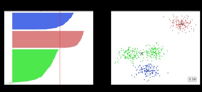
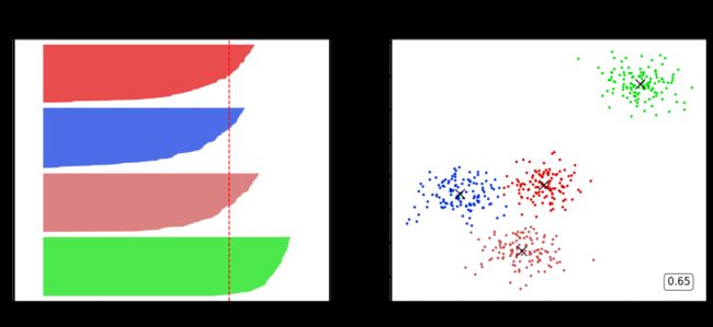
推广到循环

因为我们前面用n_clusters代替了4，所以循环for后面的变量就可以是n_clusters

for n_clusters in range(2,8,1):
    cluster = KMeans(n_clusters=n_clusters,random_state=10).fit(X)
    cluster_labels = cluster.labels_
    silhouette_avg = silhouette_score(X,cluster_labels)
    sample_silhouette_values = silhouette_samples(X,cluster_labels)
    fig,(ax1,ax2) = plt.subplots(1,2)
    fig.set_size_inches(18,7)
	
    ax1.set_xlim([-0.1,1])
    ax1.set_ylim([0,X.shape[0] + (n_clusters + 1) * 10])
	
    y_lower = 10
    
    for i in range(n_clusters):
        ith_cluster_silhouette_values = sample_silhouette_values[cluster_labels == i]
        ith_cluster_silhouette_values.sort()
        size_cluster_i = ith_cluster_silhouette_values.shape[0]
		
        y_upper = y_lower + size_cluster_i
		
        color = cm.nipy_spectral(np.random.RandomState(i+3).random(1))
		
        ax1.fill_betweenx(np.arange(y_lower,y_upper,1)
                        ,ith_cluster_silhouette_values
                        ,0
                        ,facecolor=color
                        ,alpha=0.7)
		
        y_lower = y_upper + 10
		
        ax2.scatter(X[cluster_labels == i,0],X[cluster_labels == i,1]
                   ,marker='o'
                   ,s=8
                   ,c=color)
    
    ax1.text(-0.05
             ,y_lower + 0.5 * size_cluster_i
             ,str(i))
    ax1.set_title("The silhouette plot for the various clusters.")
    ax1.set_xlabel("The silhouette coefficient values")
    ax1.set_ylabel("Cluster label")
    ax1.axvline(x=silhouette_avg,color='red',linestyle='--')
    ax1.set_yticks([])
    ax1.set_xticks([-0.1,0,0.2,0.4,0.6,0.8,1])    
    centers =cluster.cluster_centers_
    ax2.scatter(centers[:,0],centers[:,1],marker='x',c='k',s=200)
    ax2.set_title("The visualization of the clustered data.")
    ax2.set_xlabel("Feature space for the 1st feature")
    ax2.set_ylabel("Feature space for the 2nd feature")
    ax2.text(0.95, 0.06
       ,('%.2f' %silhouette_avg)
       ,size=15
       ,bbox=dict(boxstyle='round',alpha=0.8,facecolor='white')
       ,transform=ax2.transAxes
       ,horizontalalignment='right') # 借用一下支持向量机的
    plt.suptitle(("Silhouette analysis for KMeans clustering on sample data with n_clusters = %d" % n_clusters)
                 ,fontsize=14, fontweight='bold')
    plt.show()

部分代码和视频中不一样但目标是一样的

观察我们可以发现分成两簇的轮廓系数高于分成四簇的，但是在实际业务中，我们未必是选择轮廓系数最高的，需要结合实际情况