机器学习—分类算法的对比实验
文章目录
- 前言
- 一、分类算法实现
-
- 1.决策树
- 2.KNN
- 3.SVM
- 4.逻辑回归
- 5.朴素贝叶斯
- 6.随机森林
- 7.AdaBoost
- 8.GradientBoosting
- 二、分类算法的对比
前言
对各种机器学习分类算法进行对比,以鸢尾花数据集为例,我们从绘制的分类边界效果以及实验评估指标(Precision、Recall、F1-socre)分别进行对比。
代码前部分组成:
# 第一步,数据准备
from sklearn import datasets          # 引入iris数据
import numpy as np
iris = datasets.load_iris()
X = iris.data[:,[2,3]]
y = iris.target
# print(iris.data)
print("Class labels:",np.unique(y))   # 打印分类类别的种类 [0 1 2]

# 第二步,切分训练数据和测试数据
from sklearn.model_selection import train_test_split
# 30%测试数据,70%训练数据,stratify=y表示训练数据和测试数据具有相同的类别比例
X_train,X_test,y_train,y_test = train_test_split(X,y,test_size=0.3,random_state=1,stratify=y) # 随机分配训练和测试数据集

# 第三步,数据标准化
from sklearn.preprocessing import StandardScaler
sc = StandardScaler() # 估算训练数据中的mu和sigma
sc.fit(X_train)       # 使用训练数据中的mu和sigma对数据进行标准化
X_train_std = sc.transform(X_train)
X_test_std = sc.transform(X_test)

# 第四步,定制可视化函数:画出决策边界图(取2个特征才比较容易画出来)
import matplotlib.pyplot as plt
from matplotlib.colors import ListedColormap

def plot_decision_region(X,y,classifier,resolution=0.02):
    markers = ('s','x','o','^','v')
    colors = ('red','blue','lightgreen','gray','cyan')
    cmap = ListedColormap(colors[:len(np.unique(y))])

    # plot the decision surface
    x1_min,x1_max = X[:,0].min()-1,X[:,0].max()+1
    x2_min,x2_max = X[:,1].min()-1,X[:,1].max()+1
    xx1,xx2 = np.meshgrid(np.arange(x1_min,x1_max,resolution),
                         np.arange(x2_min,x2_max,resolution))
    Z = classifier.predict(np.array([xx1.ravel(),xx2.ravel()]).T)
    Z = Z.reshape(xx1.shape)
    plt.contourf(xx1,xx2,Z,alpha=0.3,cmap=cmap)
    plt.xlim(xx1.min(),xx1.max())
    plt.ylim(xx2.min(),xx2.max())

    # plot class samples
    for idx,cl in enumerate(np.unique(y)):
        plt.scatter(x=X[y==cl,0],
                   y = X[y==cl,1],
                   alpha=0.8,
                   c=colors[idx],
                   marker = markers[idx],
                   label=cl,
                   edgecolors='black')
一、分类算法实现
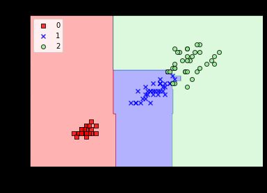
1.决策树
核心代码为:
#第四步 决策树分类
from sklearn.tree import DecisionTreeClassifier
from sklearn import metrics
tree = DecisionTreeClassifier(criterion='gini',max_depth=4,random_state=1)
tree.fit(X_train_std,y_train)
print(X_train_std.shape, X_test_std.shape, len(y_train), len(y_test)) #(105, 2) (45, 2) 105 45
res1 = tree.predict(X_test_std)
print('y_test=')
print(y_test)
print('predict=')
print(res1)
print(metrics.classification_report(y_test, res1, digits=4)) #四位小数

plot_decision_region(X_train_std,y_train,classifier=tree,resolution=0.02)
plt.xlabel('petal length [standardized]')
plt.ylabel('petal width [standardized]')
plt.title('DecisionTreeClassifier')
plt.legend(loc='upper left')
plt.show()
实验的精确率、召回率和F1值输出如下:
- macro avg 0.9792 0.9778 0.9778
y_test=
[2 0 0 2 1 1 2 1 2 0 0 2 0 1 0 1 2 1 1 2 2 0 1 2 1 1 1 2 0 2 0 0 1 1 2 2 0
 0 0 1 2 2 1 0 0]
predict=
[2 0 0 1 1 1 2 1 2 0 0 2 0 1 0 1 2 1 1 2 2 0 1 2 1 1 1 2 0 2 0 0 1 1 2 2 0
 0 0 1 2 2 1 0 0]
              precision    recall  f1-score   support

           0     1.0000    1.0000    1.0000        15
           1     0.9375    1.0000    0.9677        15
           2     1.0000    0.9333    0.9655        15

    accuracy                         0.9778        45
   macro avg     0.9792    0.9778    0.9778        45
weighted avg     0.9792    0.9778    0.9778        45
实验散点图为:

2.KNN
核心代码部分:
#第四步 KNN分类
from sklearn.neighbors import KNeighborsClassifier
from sklearn import metrics
knn = KNeighborsClassifier(n_neighbors=2,p=2,metric="minkowski")
knn.fit(X_train_std,y_train)
res2 = knn.predict(X_test_std)
print('y_test=')
print(y_test)
print('predict=')
print(res2)
print(metrics.classification_report(y_test, res2, digits=4)) #四位小数

plot_decision_region(X_train_std,y_train,classifier=knn,resolution=0.02)
plt.xlabel('petal length [standardized]')
plt.ylabel('petal width [standardized]')
plt.title('KNeighborsClassifier')
plt.legend(loc='upper left')
plt.show()
实验的精确率、召回率和F1值输出如下:
- macro avg 0.9792 0.9778 0.9778
y_test=
[2 0 0 2 1 1 2 1 2 0 0 2 0 1 0 1 2 1 1 2 2 0 1 2 1 1 1 2 0 2 0 0 1 1 2 2 0
 0 0 1 2 2 1 0 0]
predict=
[2 0 0 1 1 1 2 1 2 0 0 2 0 1 0 1 2 1 1 2 2 0 1 2 1 1 1 2 0 2 0 0 1 1 2 2 0
 0 0 1 2 2 1 0 0]
              precision    recall  f1-score   support

           0     1.0000    1.0000    1.0000        15
           1     0.9375    1.0000    0.9677        15
           2     1.0000    0.9333    0.9655        15

    accuracy                         0.9778        45
   macro avg     0.9792    0.9778    0.9778        45
weighted avg     0.9792    0.9778    0.9778        45
实验散点图为:

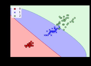
3.SVM
核心代码部分:
#第四步 SVM分类 核函数对非线性分类问题建模(gamma=0.20)
from sklearn.svm import SVC
from sklearn import metrics
svm = SVC(kernel='rbf',random_state=1,gamma=0.20,C=1.0) #较小的gamma有较松的决策边界
svm.fit(X_train_std,y_train)
res3 = svm.predict(X_test_std)
print('y_test=')
print(y_test)
print('predict=')
print(res3)
print(metrics.classification_report(y_test, res3, digits=4))

plot_decision_region(X_train_std,y_train,classifier=svm,resolution=0.02)
plt.xlabel('petal length [standardized]')
plt.ylabel('petal width [standardized]')
plt.title('SVM')
plt.legend(loc='upper left')
plt.show()
实验的精确率、召回率和F1值输出如下:
- macro avg 0.9361 0.9333 0.9340
y_test=
[2 0 0 2 1 1 2 1 2 0 0 2 0 1 0 1 2 1 1 2 2 0 1 2 1 1 1 2 0 2 0 0 1 1 2 2 0
 0 0 1 2 2 1 0 0]
predict=
[2 0 0 1 1 1 2 1 2 0 0 2 0 1 0 1 2 1 1 2 2 0 1 2 1 1 1 2 0 2 0 0 1 1 2 2 0
 0 0 1 2 2 1 0 0]
              precision    recall  f1-score   support

           0     1.0000    0.9333    0.9655        15
           1     0.9333    0.9333    0.9333        15
           2     0.8750    0.9333    0.9032        15

    accuracy                         0.9333        45
   macro avg     0.9361    0.9333    0.9340        45
weighted avg     0.9361    0.9333    0.9340        45
实验散点图为:
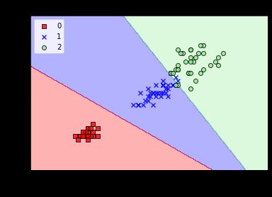
4.逻辑回归
核心代码部分:
#第四步 逻辑回归分类
from sklearn.linear_model import LogisticRegression
from sklearn import metrics
lr = LogisticRegression(C=100.0,random_state=1)
lr.fit(X_train_std,y_train)
res4 = lr.predict(X_test_std)
print('y_test=')
print(y_test)
print('predict=')
print(res4)
print(metrics.classification_report(y_test, res4, digits=4))

plot_decision_region(X_train_std,y_train,classifier=lr,resolution=0.02)
plt.xlabel('petal length [standardized]')
plt.ylabel('petal width [standardized]')
plt.title('LogisticRegression')
plt.legend(loc='upper left')
plt.show()
实验的精确率、召回率和F1值输出如下:
- macro avg 0.9792 0.9778 0.9778
y_test=
[2 0 0 2 1 1 2 1 2 0 0 2 0 1 0 1 2 1 1 2 2 0 1 2 1 1 1 2 0 2 0 0 1 1 2 2 0
 0 0 1 2 2 1 0 0]
predict=
[2 0 0 1 1 1 2 1 2 0 0 2 0 1 0 1 2 1 1 2 2 0 1 2 1 1 1 2 0 2 0 0 1 1 2 2 0
 0 0 1 2 2 1 0 0]
              precision    recall  f1-score   support

           0     1.0000    1.0000    1.0000        15
           1     0.9375    1.0000    0.9677        15
           2     1.0000    0.9333    0.9655        15

    accuracy                         0.9778        45
   macro avg     0.9792    0.9778    0.9778        45
weighted avg     0.9792    0.9778    0.9778        45
实验散点图为:
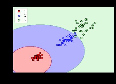
5.朴素贝叶斯
核心代码部分:
#第四步 朴素贝叶斯分类
from sklearn.naive_bayes import GaussianNB
from sklearn import metrics
gnb = GaussianNB()
gnb.fit(X_train_std,y_train)
res5 = gnb.predict(X_test_std)
print('y_test=')
print(y_test)
print('predict=')
print(res5)
print(metrics.classification_report(y_test, res5, digits=4))

plot_decision_region(X_train_std,y_train,classifier=gnb,resolution=0.02)
plt.xlabel('petal length [standardized]')
plt.ylabel('petal width [standardized]')
plt.title('GaussianNB')
plt.legend(loc='upper left')
plt.show()
实验的精确率、召回率和F1值输出如下:
- macro avg 0.9792 0.9778 0.9778
y_test=
[2 0 0 2 1 1 2 1 2 0 0 2 0 1 0 1 2 1 1 2 2 0 1 2 1 1 1 2 0 2 0 0 1 1 2 2 0
 0 0 1 2 2 1 0 0]
predict=
[2 0 0 1 1 1 2 1 2 0 0 2 0 1 0 1 2 1 1 2 2 0 1 2 1 1 1 2 0 2 0 0 1 1 2 2 0
 0 0 1 2 2 1 0 0]
              precision    recall  f1-score   support

           0     1.0000    1.0000    1.0000        15
           1     0.9375    1.0000    0.9677        15
           2     1.0000    0.9333    0.9655        15

    accuracy                         0.9778        45
   macro avg     0.9792    0.9778    0.9778        45
weighted avg     0.9792    0.9778    0.9778        45
实验散点图为:
6.随机森林
核心代码部分:
#第四步 随机森林分类
from sklearn.ensemble import RandomForestClassifier
from sklearn import metrics
forest = RandomForestClassifier(criterion='gini',
                                n_estimators=25,
                                random_state=1,
                                n_jobs=2,
                                verbose=1)
forest.fit(X_train_std,y_train)
res6 = gnb.predict(X_test_std)
print('y_test=')
print(y_test)
print('predict=')
print(res6)
print(metrics.classification_report(y_test, res6, digits=4))

plot_decision_region(X_train_std,y_train,classifier=forest,resolution=0.02)
plt.xlabel('petal length [standardized]')
plt.ylabel('petal width [standardized]')
plt.title('GaussianNB')
plt.legend(loc='upper left')
plt.show()
实验的精确率、召回率和F1值输出如下:
- macro avg 0.9792 0.9778 0.9778
y_test=
[2 0 0 2 1 1 2 1 2 0 0 2 0 1 0 1 2 1 1 2 2 0 1 2 1 1 1 2 0 2 0 0 1 1 2 2 0
 0 0 1 2 2 1 0 0]
predict=
[2 0 0 1 1 1 2 1 2 0 0 2 0 1 0 1 2 1 1 2 2 0 1 2 1 1 1 2 0 2 0 0 1 1 2 2 0
 0 0 1 2 2 1 0 0]
              precision    recall  f1-score   support

           0     1.0000    1.0000    1.0000        15
           1     0.9375    1.0000    0.9677        15
           2     1.0000    0.9333    0.9655        15

    accuracy                         0.9778        45
   macro avg     0.9792    0.9778    0.9778        45
weighted avg     0.9792    0.9778    0.9778        45
实验散点图为:
7.AdaBoost
Adaboost算法
boosting算法中的一个典型代表——Adaboost算法。简单来说,Adaboost算法还是按照boosting算法的思想,要建立多个基础模型,一个个地串联在一起。
核心代码部分:
#第四步 集成学习分类
from sklearn.ensemble import AdaBoostClassifier
from sklearn import metrics
ada = AdaBoostClassifier()
ada.fit(X_train_std,y_train)
res7 = ada.predict(X_test_std)
print('y_test=')
print(y_test)
print('predict=')
print(res7)
print(metrics.classification_report(y_test, res7, digits=4))

plot_decision_region(X_train_std,y_train,classifier=forest,resolution=0.02)
plt.xlabel('petal length [standardized]')
plt.ylabel('petal width [standardized]')
plt.title('AdaBoostClassifier')
plt.legend(loc='upper left')
plt.show()
实验的精确率、召回率和F1值输出如下:
- macro avg 0.9792 0.9778 0.9778
y_test=
[2 0 0 2 1 1 2 1 2 0 0 2 0 1 0 1 2 1 1 2 2 0 1 2 1 1 1 2 0 2 0 0 1 1 2 2 0
 0 0 1 2 2 1 0 0]
predict=
[2 0 0 1 1 1 2 1 2 0 0 2 0 1 0 1 2 1 1 2 2 0 1 2 1 1 1 2 0 2 0 0 1 1 2 2 0
 0 0 1 2 2 1 0 0]
              precision    recall  f1-score   support

           0     1.0000    1.0000    1.0000        15
           1     0.9375    1.0000    0.9677        15
           2     1.0000    0.9333    0.9655        15

    accuracy                         0.9778        45
   macro avg     0.9792    0.9778    0.9778        45
weighted avg     0.9792    0.9778    0.9778        45
实验散点图为:

8.GradientBoosting
核心代码部分:
#第四步 GradientBoosting分类
from sklearn.ensemble import GradientBoostingClassifier
from sklearn import metrics
gb = GradientBoostingClassifier()
ada.fit(X_train_std,y_train)
res8 = ada.predict(X_test_std)
print('y_test=')
print(y_test)
print('predict=')
print(res8)
print(metrics.classification_report(y_test, res8, digits=4))

plot_decision_region(X_train_std,y_train,classifier=forest,resolution=0.02)
plt.xlabel('petal length [standardized]')
plt.ylabel('petal width [standardized]')
plt.title('GradientBoostingClassifier')
plt.legend(loc='upper left')
plt.show()
实验的精确率、召回率和F1值输出如下:
- macro avg 0.9792 0.9778 0.9778
y_test=
[2 0 0 2 1 1 2 1 2 0 0 2 0 1 0 1 2 1 1 2 2 0 1 2 1 1 1 2 0 2 0 0 1 1 2 2 0
 0 0 1 2 2 1 0 0]
predict=
[2 0 0 1 1 1 2 1 2 0 0 2 0 1 0 1 2 1 1 2 2 0 1 2 1 1 1 2 0 2 0 0 1 1 2 2 0
 0 0 1 2 2 1 0 0]
              precision    recall  f1-score   support

           0     1.0000    1.0000    1.0000        15
           1     0.9375    1.0000    0.9677        15
           2     1.0000    0.9333    0.9655        15

    accuracy                         0.9778        45
   macro avg     0.9792    0.9778    0.9778        45
weighted avg     0.9792    0.9778    0.9778        45
实验散点图为:

二、分类算法的对比
对数据结果进行比较,由于数据较少差距情况不是很明显,从而不是很明显可以看出来,但是方法是类似的。
对比情况:
| 分类算法 | precision | recall | f1-score |
|---|---|---|---|
| 决策树 | 0.9792 | 0.9778 | 0.9778 |
| KNN | 0.9792 | 0.9778 | 0.9778 |
| SVM | 0.9361 | 0.9333 | 0.9340 |
| 逻辑回归 | 0.9792 | 0.9778 | 0.9778 |
| 朴素贝叶斯 | 0.9792 | 0.9778 | 0.9778 |
| 随机森林 | 0.9792 | 0.9778 | 0.9778 |
| AdaBoost | 0.9792 | 0.9778 | 0.9778 |
| GradientBoosting | 0.9792 | 0.9778 | 0.9778 |
对比图:
