Multivariate Linear Regression
Multivariate Linear Regression
Multiple Features
Multivariate linear regression: Linear regression with mutiple variables.
Notation
n n n= number of features
x ( i ) x^{(i)} x(i)= input (features) of i t h i^{th} ith training example.
x j i x_j^{i} xji= value of feature j j j in i t h i^{th} ith training example.
h θ ( x ) h_\theta(x) hθ(x)= θ 0 + θ 1 x 1 + . . . θ n x n \theta_0+\theta_1x_1+...\theta_nx_n θ0+θ1x1+...θnxn
For convenience of notation, define x 0 x_0 x0=1.(That is, x 0 ( i ) x_0^{(i)} x0(i)=1)
x = [ x 0 x 1 ⋯ x n ] ∈ R n + 1 x=\begin{bmatrix} x_0\\x_1\\\cdots\\x_n \end{bmatrix}\in\R^{n+1} x=⎣⎢⎢⎡x0x1⋯xn⎦⎥⎥⎤∈Rn+1
θ = [ θ 0 θ 1 ⋯ θ n ] ∈ R n + 1 \theta=\begin{bmatrix} \theta_0\\\theta_1\\\cdots\\\theta_n\end{bmatrix}\in\R^{n+1} θ=⎣⎢⎢⎡θ0θ1⋯θn⎦⎥⎥⎤∈Rn+1
h θ ( x ) h_\theta(x) hθ(x)= θ T x \theta^Tx θTx
Gradient Descent for Multiple Variable
The gradient descent equation is generally the same form, we just have to repeat it for ‘n’ features:
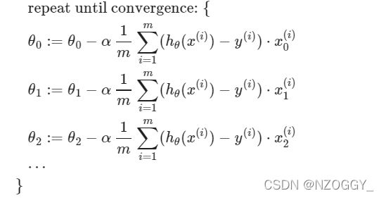
Repeat until convergence:{
θ j \theta_j θj:= θ j \theta_j θj- α 1 m ∑ i = 1 m ( h θ ( x ( i ) ) − y ( i ) ) ⋅ x j ( i ) \alpha\frac{1}{m}\sum^m_{i=1}{(h_\theta(x^{(i)} )-y^{(i)})\cdot x_j^{(i)} } αm1∑i=1m(hθ(x(i))−y(i))⋅xj(i)
}
Gradient Descent in Practice I- Feature Scaling
Idea: Make sure features are on similar scale.
Modify the ranges of our input variables: Speed up gradient descent by having each of input values in roughly the same range.(make the contour of cost function J J J can become less skewed)
Because θ \theta θ will descend quickly on small ranges and slowly on large ranges. This will oscillate inefficiently down to the optimum when the variables are very uneven.
No exact requirements.
Two techniques:
feature scaling :Dividing the input values by the range of the input variables
Get every feature into approximately a − 1 ≤ x i ≤ 1 -1\leq x_i\leq1 −1≤xi≤1 range.
mean normalization: Subtracting the average value for an input variable from the values for that input variable.
Replace x i x_i xi with x i − μ i x_i-\mu_i xi−μi to make features have approximately zero mean (Do not apply to x 0 = 1 x_0=1 x0=1)
Adjust input values in the formula:
x i : = x i − μ i s i x_i :=\frac{x_i-\mu_i}{s_i} xi:=sixi−μi
μ \mu μ is the average of all the values for features(i) and s i s_i si is the range of values (max-min), or s i s_i si is the standard deviation.
- Dividing by the range, or dividing by the standard deviation, give different results.
Gradient Descent in Practice II- Learning Rate
- Debugging gradient descent
Make a plot with number of iterations on the x-axis. Now plot the cost function, J(θ) over the number of iterations of gradient descent. If J( θ \theta θ) ever increases, then we need to increase α \alpha α.
( J θ J_\theta Jθ should decrease after every iteration)
- Automatic convergence test
Declare convergence if J(θ) decreases by less than E in one iteration, where E is some small value such as 1 0 − 3 10^{−3} 10−3.
If learning rate α is sufficiently small, then J(θ) will decrease on every iteration.
If α is too small: slow convergence.
If α is too large: may not decrease on every iteration and thus may not converge.
Features and Polynomial Regression
Improve features and the form of hypothesis
- combine multiple features into one
Polynomial Regression
- change the behavior or curve
(making it a quadratic, cubic or square root function (or any other form))
Keep in mind that, if you choose your features this way then feature scaling becomes very important.