利用CNN对MNIST训练

目录

1 简介

2 数据集

3 数据预处理

3.1 数据集导入

3.2 像素值归一化处理

3.3 计算图片的高和宽

3.4 读取标签并进行one-hot编码

3.5 数据集划分

4 参数与网络设置

4.1 参数设置

4.2 网络设置

5 损失设置与训练

6 结果展示

---

1 简介

MNIST是一个入门级的计算机视觉数据集，它包含各种从0到9的手写数字图片以及对应的标签，本篇使用了简单卷积神经网络来实现手写图片预测，主要目的在于熟悉CNN的操作。

首先，设置一些参数

%matplotlib inline
import matplotlib.pyplot as plt
import matplotlib.cm as cm
import numpy as np
import pandas as pd
import tensorflow as tf
​
# 设置
# 学习率
Learning_Rate = 1e-4
# 训练轮数
Training_Iterations = 2500
# dropout保留百分比
Dropout = 0.6
# 批处理数量
Batch_Size = 50
# 测试数据集数量
Validation_Size = 2000
# 前期测试展示图像编号
Image_To_Display = 10

2 数据集

本次使用了mnist的csv格式的数据，通过原版的train-images-idx3-ubyte.gz、train-labels-idx1-ubyte.gz、t10k-images-idx3-ubyte.gz、t10k-labels-idx1-ubyte.gz转换，此数据集训练数据共60000条，本次训练只使用了训练数据集，其中58000条作为训练数据，2000条作为测试数据：

def convert(imgf, labelf, outf, n):
    #rb，以二进制只读方式从文件开头打开
    #w，从文件开头开始写入
    f = open(imgf, "rb")
    o = open(outf, "w")
    l = open(labelf, "rb")
​
    # 读入指定字节数
    f.read(16)
    l.read(8)
​
    # 创建一个列表
    images = []
​
    for i in range(n):
        # ord()返回字符对应的ASC码
        image = [ord(l.read(1))]    #添加标签
        
        for j in range(28*28):
            image.append(ord(f.read(1)))    #添加图像
        
        images.append(image)    #存入列表
​
    #写入输出文件
    #写入列名，label,pixel0,pixel1...piexl783
    o.write("label,")
    pixel = []
    for p in range(28*28):
        name = "pixel" + str(p)
        pixel.append(name)
        
    o.write(",".join(pixel))
    o.write("\n")
    #写入图像数据
    for image in images:
        o.write(",".join(str(pix) for pix in image)+"\n")
    f.close()
    o.close()
    l.close()
​
#生成train.csv
convert(r"路径\train-images.idx3-ubyte", r"路径\train-labels.idx1-ubyte",
        r"路径\mnist_train.csv", 60000)
​
#生成test.csv
convert(r"路径\t10k-images.idx3-ubyte", r"路径\t10k-labels.idx1-ubyte",
        r"路径\mnist_test.csv", 10000)
​
print("Convert Finished!")

注意事项：

• 文件读入与保存时，路径前加r，或者使用\\，防止了\n的转义，否则无法执行。

• 必须写列名，后面数据集读入后才能通过列名读取数据，否则读取失败。

转换后的数据：

 

3 数据预处理

3.1 数据集导入

# 导入文件
data = pd.read_csv('mnist_train.csv')
​
print('data({0[0]},{0[1]})'.format(data.shape))
print(data.head())

通过pandas包导入csv文件，输出如下：

 

若转换csv文件时没有写入列名，此时列名会变成一些奇奇怪怪的数，其后面读取标签时找不到index。

3.2 像素值归一化处理

# 图像的灰度值在0~255之间，差异性过大，先进行归一化处理
images = data.iloc[:,1:].values
images = images.astype(np.float)
​
images = np.multiply(images, 1.0 / 255.0)
​
print('images({0[0]},{0[1]})'.format(images.shape))

图像的像素值在0~255之间，数值的差异性过大，不利于模型的训练，因此先进行归一化处理，将像素值从0~255转换成0~1。

3.3 计算图片的高和宽

# 此时图像是一个784的长条，需要转换成28x28的，先算出来高和宽的值
image_size = images.shape[1]
print('image_size = {0}'.format(image_size))
​
image_width = image_height = np.ceil(np.sqrt(image_size)).astype(np.uint8)
print('image_width = {0}\nimage_height = {1}'.format(image_width,image_height))

csv数据集中每张图片都是1x784的，训练时需要转换成28x28的，因此先计算出转换后的高和宽(28)

可以进行一下图片展示(此步可跳过)：

def display(img):
    
    one_image = img.reshape(image_width,image_height)
    
    plt.axis('off')
    plt.imshow(one_image, cmap=cm.binary)
​
display(images[Image_To_Display])

 

3.4 读取标签并进行one-hot编码

读取标签：

# 读取标签数据和类型数量
labels_flat = data['label'].values.ravel()
labels_count = np.unique(labels_flat).shape[0]
​
print('labels_flat({0})'.format(len(labels_flat)))
print('labels_flat[{0}] = {1}'.format(Image_To_Display, labels_flat[Image_To_Display]))
print('labels_count = {0}'.format(labels_count))

 

此时标签仅为一个数字，该数字为图片的标签，但是训练中需要用到分别为各类数字的几率，因此需要进行ont-hot编码，即0→[1,0,0,0,0,0,0,0,0,0], 1→[0,1,0,0,0,0,0,0,0,0],..., 9→[0,0,0,0,0,0,0,0,0,1]，某一个数字类型的概率为1，其他类型的概率为0。

# 对标签进行one-hot coding
# 0 => [1,0,0,0,0,0,0,0,0,0]
# 1 => [0,1,0,0,0,0,0,0,0,0]
# ...
# 9 => [0,0,0,0,0,0,0,0,0,1]
​
def dense_to_one_hot(labels_dense, num_classes):
    num_labels = labels_dense.shape[0]    # 样本数量
    index_offset = np.arange(num_labels) * num_classes  # [0,10,20,...,599990]
    labels_one_hot = np.zeros((num_labels, num_classes))
    labels_one_hot.flat[index_offset + labels_dense.ravel()] = 1
    return labels_one_hot
    
labels = dense_to_one_hot(labels_flat, labels_count)
labels = labels.astype(np.uint8)
​
print('labels({0[0]},{0[1]})'.format(labels.shape))
print('labels[{0}] = {1}'.format(Image_To_Display, labels[Image_To_Display]))

此处的labels[10]是上面展示的‘3’的手写数字的标签，是3的概率为1，是其他数字的概率为0。

3.5 数据集划分

本次训练只使用了mnist数据集中的训练数据集，共60000条，其中前2000条作为测试数据，后58000条作为训练数据：

validation_images = images[:Validation_Size]  #前2000作为测试数据
validation_labels = labels[:Validation_Size]
​
train_images = images[Validation_Size:]
train_labels = labels[Validation_Size:]
​
print('train_images({0[0]},{0[1]})'.format(train_images.shape))
print('validation_images({0[0]},{0[1]})'.format(validation_images.shape))

 

4 参数与网络设置

4.1 参数设置

定义两个方法，自动生成权重与偏置：

# 权重与偏置
def weight_variable(shape):
    initial = tf.truncated_normal(shape, stddev=0.1)  # 高斯初始化
    return tf.Variable(initial)
​
def bias_variable(shape):
    initial = tf.constant(0.1, shape=shape)
    return tf.Variable(initial)

指定卷积操作，步长为1：

# 指定卷积操作
def conv2d(x, W):
    return tf.nn.conv2d(x, W, strides=[1,1,1,1], padding='SAME')

#strides=[batch_size(在batchsize上是否有滑动), 图像的高, 图像的宽, 图像的通道(RGB)]

指定池化操作(2x2,strides=2)：

# 指定池化操作
def max_pool_2x2(x):
    return tf.nn.max_pool(x, ksize=[1, 2, 2, 1], strides=[1, 2, 2, 1], padding='SAME')

指定输入输出：

# 指定输入输出
x = tf.placeholder('float', shape=[None, image_size])
y_ = tf.placeholder('float', shape=[None, labels_count])

4.2 网络设置

本次网络结构为：输入→卷积(32)→池化→卷积(64)→池化→全连接(1024)→输出(10)

网络构造如下：

 

第一层：

# 指定神经网络模型
# 第一层
W_conv1 = weight_variable([5, 5, 1, 32]) # filter为5x5x1,32个
b_conv1 = bias_variable([32])
​
# (58000,784) => (58000,28,28,1)
image = tf.reshape(x, [-1, image_width, image_height, 1])
# -1表示未知数，自动求解
​
h_conv1 = tf.nn.relu(conv2d(image, W_conv1) + b_conv1) # 卷积层
# h_conv1.get_shape() = (58000, 28, 28, 32)
h_pool1 = max_pool_2x2(h_conv1)                        # 池化层
# h_pool1.get_shape() = (58000, 14, 14, 32)

第二层：

# 第二层
W_conv2 = weight_variable([5, 5, 32, 64]) # 经过一次pooling，filter个数翻倍
b_conv2 = bias_variable([64])
​
h_conv2 = tf.nn.relu(conv2d(h_pool1, W_conv2) + b_conv2)
# h_conv2.get_shape() = (58000, 14, 14, 64)
h_pool2 = max_pool_2x2(h_conv2)
# h_pool2.get_shape() = (58000, 7, 7, 64)

全连接层：

# 指定全连接层
W_fc1 = weight_variable([7*7*64, 1024])
b_fc1 = bias_variable([1024])
​
# 将特征提取结果展开  (58000, 7, 7, 64) => (58000, 3136)
h_pool2_flat = tf.reshape(h_pool2, [-1, 7*7*64])
​
h_fc1 = tf.nn.relu(tf.matmul(h_pool2_flat, W_fc1) + b_fc1)
# h_fc1.get_shape() = (58000, 1024)

指定dropout：

# 指定dropout, 一般只加在最后的几层全连接层
keep_prob = tf.placeholder('float')
h_fc1_drop = tf.nn.dropout(h_fc1, keep_prob)

得到结果：

# 得到结果
W_fc2 = weight_variable([1024, labels_count])
b_fc2 = bias_variable([labels_count])
​
y = tf.nn.softmax(tf.matmul(h_fc1_drop, W_fc2) + b_fc2)
# y.getshape() = (58000,10)

5 损失设置与训练

设置损失函数与评估参数：

# 损失函数
cross_entropy = -tf.reduce_sum(y_*tf.log(y))
​
# 优化器
train_step = tf.train.GradientDescentOptimizer(Learning_Rate).minimize(cross_entropy)
​
# 评估
correct_prediction = tf.equal(tf.argmax(y,1), tf.argmax(y_,1))
accuracy = tf.reduce_mean(tf.cast(correct_prediction, 'float'))
predict = tf.argmax(y,1)

定义批读入方法next_batch:

epochs_completed = 0
index_in_epoch = 0
num_examples = train_images.shape[0]
​
# 批读入数据，定好起始地址、终止地址然后拿数据就好
def next_batch(batch_size):
    
    global train_images
    global train_labels
    global index_in_epoch
    global epochs_completed
    
    start = index_in_epoch
    index_in_epoch += batch_size
    
    if index_in_epoch > num_examples:
        # 一轮结束
        epochs_completed += 1
        # 刷新数据集
        perm = np.arange(num_examples)
        np.random.shuffle(perm)
        train_images = train_images[perm]
        train_labels = train_labels[perm]
        # 开始下一轮
        start = 0
        index_in_epoch = batch_size
        assert batch_size <= num_examples
    end = index_in_epoch
    return train_images[start:end], train_labels[start:end]

开始训练：

# 初始化
init = tf.global_variables_initializer()
sess = tf.InteractiveSession()
sess.run(init)
​
# 开始训练
train_accuracies = []        #后面用来画图
validation_accuracies = []
x_range = []
​
display_step = 1   # 采用动态输出，每输出10次，step*10，见下面
​
for i in range(Training_Iterations):
    
    # 批读入数据
    batch_xs, batch_ys = next_batch(Batch_Size)
    
    # 展示
    if (i+1)%display_step == 0 or (i+1) == Training_Iterations:
        # 训练数据精度
        train_accuracy = accuracy.eval(feed_dict={x:batch_xs,
                                                   y_:batch_ys,
                                                   keep_prob: 1.0})
        #测试数据精度
        if(Validation_Size):
            validation_accuracy = accuracy.eval(feed_dict={x:validation_images[0:Batch_Size],
                                                             y_:validation_labels[0:Batch_Size],
                                                             keep_prob: 1.0})
            # keep_prob 是 dropout 的设置
            
            print(' training accuracy / validation accuracy = %.2f / %.2f for step %d' % (train_accuracy, validation_accuracy, i+1))
            
            validation_accuracies.append(validation_accuracy)
            
        else:
            print(' training accuracy = %.2f for step %d' % (train_accuracy, i+1))
        
        train_accuracies.append(train_accuracy)
        x_range.append(i+1)
        
        # 展示间隔增加
        if (i+1)%(display_step*10) == 0 and i:
            display_step *= 10
    # 开始
    sess.run(train_step, feed_dict={x:batch_xs, y_:batch_ys, keep_prob: Dropout})

6 结果展示

结果可通过图表显示：

# 结果展示表
if(Validation_Size):
    validation_accuracy = accuracy.eval(feed_dict={x:validation_images[0:Batch_Size],
                                                             y_:validation_labels[0:Batch_Size],
                                                             keep_prob: 0.6})
    print(' validation accuracy = %.4f' % validation_accuracy)
    plt.plot(x_range, train_accuracies, '-b', label='Training')
    plt.plot(x_range, validation_accuracies, '-g', label='Validation')
    plt.legend(loc='lower right', frameon=False)
    plt.ylim(ymax = 1.1, ymin = 0.7)
    plt.ylabel('accuracy')
    plt.xlabel('step')
    plt.show()

本次使用的学习率为0.0001，dropout为0.6：

 

 

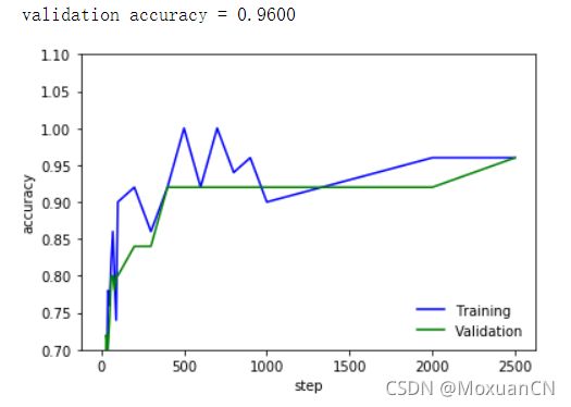
总体精度从300~400轮左右开始超过90%，后面很多轮都是92%左右，最后2000~2500轮大概为96%。

此外，还增加了卷积核的数量进行了一次训练，网络构成为：

输入→卷积(64)→池化→卷积(128)→池化→全连接(1024)→输出(10)

训练结果为：

 

 

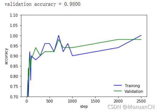
总体精度从100轮左右开始达到90%左右，后面慢慢提升，最后大概为98%。