RNA-seq数据分析

一、数据收集

1.NCBI GEO数据库收集相关RNA-seq数据

样本信息以及引用文献可以点击对应链接查看

2.SRA Run Selector 查看数据单双端类型（SINGLE or PAIRED)及分组信息

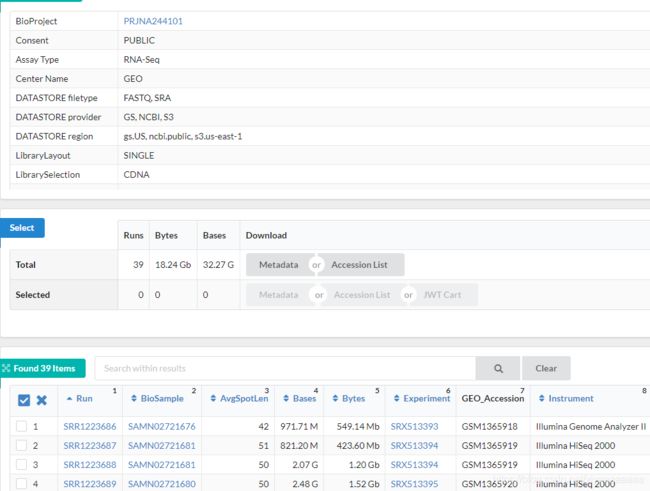
可以点击Accession List下载对应的SRR_Acc_List.txt

二、RNA-seq 处理流程

使用HISAT, StringTie and Ballgown处理流程

<一>下载并解压SRA文件

1.根据下载的SRR_Acc_List.txt下载原始sra文件至SRR文件夹

prefetch -O SRR/ --option-file SRR_Acc_List.txt

2.解压sra文件生成对应的fastq文件至fastq文件夹

for i in SRR/SRR*/*.sra; do echo $i ; fasterq-dump -O fastq/  -e  16 --split-3 $i; done
#--split-3, 会把双端sra文件拆分成两个文件,但是单端并不会保存成两个文件

<二>对数据进行质量控制

fastqc进行质控，multiqc合并质控结果

#fastqc
#fastqc质控
for i in fastq/*.fastq; do echo $i ; fastqc -t 20 -o fastq/quality $i; done
#multiqc
multiqc fastq/quality/ -n before_report.html -o fastq/

<三> 数据裁剪

1.fastp使用

#单端测序数据（single-end，SE）
fastp -i in.fq -o out.fq
#双端测序数据（paired-end，PE）
fastp -i in.R1.fq -o out.R1.fq -I in.R2.fq -O out.R2.fq

2.参数详解

#单端数据
for filename in fastq/*.fastq
do
base=$(basename $filename .fastq)
echo $base
fastp -i fastq/${base}.fastq -o fastq/deal/${base}.fastq -w 16  -x --trim_poly_x --poly_x_min_len 20 -q 20 -u 40 -n 5 -3 -W 4 -M 25
done 
#-w 16 线程数  
#-x --trim_poly_x --poly_x_min_len 20 切除polyx尾巴，尾巴长度设置为20
#-q 20 -u 40 表示一个 read 最多只能有 40%的碱基的质量值低于Q20，否则会被扔掉  
#-n 5 过滤N碱基过多的reads  
#-3 -W 4 -M 25 从3'开始移动滑动窗口，滑窗大小为4， 平均质量低于25被切

#双端数据
for filename in fastq/*_1.fastq
do
base=$(basename $filename _1.fastq)
echo $base
fastp -i fastq/${base}_1.fastq -I fastq/${base}_2.fastq -o fastq/deal/${base}_1.fastq -O fastq/deal/${base}_2.fastq -w 16  -x --trim_poly_x --poly_x_min_len 20 -q 20 -u 40 -n 5 -3 -W 4 -M 25 -c --overlap_len_require 30 --overlap_diff_limit 5 --overlap_diff_percent_limit 20
done
#-c, --correction 对PE碱基校正，使用该参数是基于检测overlap。
#--overlap_len_require overlap的长度要求，默认是30，即默认overlap区域的长度不低于30bp；
#--overlap_diff_limit overlap中最大错配数，默认是5，即默认overlap时最多有5个错配；
#--overlap_diff_percent_limit overlap中最大错配数在重叠区的占比，默认是20，即默认最大错配数的碱基占比不高于20%；否则认为无overlap。`

<四>检查数据质量

#fastqc
#fastqc质控
for i in fastq/deal/*.fastq; do echo $i ; fastqc -t 20 -o fastq/deal/quality $i; done
#multiqc
multiqc fastq/deal/quality/ -n after_report.html -o fastq/

<五>Hisat比对

1.参考基因组及对应注释文件（gtf）下载

参考基因组与注释文件要对应，否则比对率很低且下游分析比较麻烦
iGenomes

2.Hisat2索引

• 模式生物可以直接进入hisat2官网进行index下载http://daehwankimlab.github.io/hisat2/download/
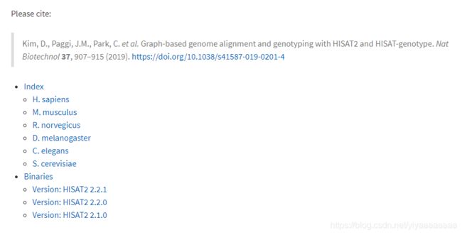
• 非模式生物需要自己建立索引

hisat2-build -p 16 genome.fa genome
#genome.fa  为对应的参考基因组
#genome 为建立的索引名称

3.mapping到参考基因组

#单端文件比对
for filename in fastq/deal/*.fastq
do
base=$(basename $filename .fastq)
echo $base
hisat2 -t -p 16 --dta -x /lustre/home/acct-clsdqw/clsdqw-user1/Desktop/RNA-seq/E.coli/reference/hisat2/genome \
-U fastq/deal/${base}.fastq -S process/sam/${base}.sam

#双端文件比对
for filename in fastq/deal/*_1.fastq
do
base=$(basename $filename _1.fastq)
echo $base
hisat2 -t -p 20 -x /lustre/home/acct-clsdqw/clsdqw-user1/Desktop/RNA-seq/code/Yeast/reference/hisat2/genome \
-1 fastq/deal/${base}_1.fastq -2 fastq/deal/${base}_2.fastq -S process/sam/${base}.sam

-x 要写到对应的索引名称

<六>samtools进行格式转换并排序

1.view: 将sam文件与bam文件互换
bam文件优点：bam文件为二进制文件，占用的磁盘空间比sam文本文件小；利用bam二进制文件的运算速度快。
2.sort: 对bam文件进行排序(sort)
这些操作是对bam文件进行的，因而当输入为sam文件的时候，不能进行该操作

samtools view -@ 16 -S process/sam/${base}.sam -b > process/bam/${base}.bam
samtools sort -@ 16 process/bam/${base}.bam -o process/bam_sort/${base}.bam

<七>得到转录本并进行组装

#获得gtf
for filename in process/bam_sort/*.bam
do
base=$(basename $filename .bam)
echo $base
stringtie -p 16 process/bam_sort/${base}.bam -G /lustre/home/acct-clsdqw/clsdqw-user1/Desktop/RNA-seq/E.coli/reference/E.coli.gtf -o process/gtf/${base}.gtf
done

#获得strimerge.gtf
for filename in process/gtf/*.gtf
do
base=$(basename $filename .gtf)
echo process/gtf/${base}.gtf >> process/gtf/mergelist.txt
done
stringtie --merge -p 16 -G /lustre/home/acct-clsdqw/clsdqw-user1/Desktop/RNA-seq/E.coli/reference/E.coli.gtf -o process/gtf/strimerge.gtf process/gtf/mergelist.txt

<八>Ballgown获得所有转录本及其丰度

#ballgown
for filename in process/bam_sort/*.bam
do
base=$(basename $filename .bam)
echo $base
stringtie -e -B -p 16 -G process/gtf/strimerge.gtf -o ballgown/${base}/${base}.gtf process/bam_sort/${base}.bam
done

三、下游分析

1.使用R语言进行差异表达基因筛选，GO KEGG富集分析并绘图

my_DEG_analysis <-function(gse_name,phenodata,ballgownfile,smallprotein,logfc,pvalue)
{

	library(ballgown)
	library(genefilter)
	library(dplyr)
	library(devtools)
	library(ggplot2)
	library(GSEABase)
  

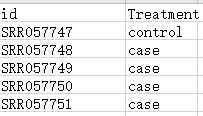
	###指定分组信息
	sampleGroup <- read.csv(phenodata, header = TRUE)
	#DESeq2说明清楚哪个因子level对应的control，避免后面解释数据遇到麻烦（你不知道到底logFC是以谁做参照的，希望是以control作为参照，这样logFC>1就表示实验组表达大于对照组；但是R不知道，R默认按字母顺序排列因子顺序，所以要对这个因子顺序set一下：
	
	#factor levels，写在前面的level作为参照
	sampleGroup$Treatment <- factor(sampleGroup$Treatment, levels = c("control", "case"))

	###读入数据
	bg_chrX=ballgown(dataDir =ballgownfile,samplePattern = "SRR", meas='all',pData=sampleGroup)
	whole_tx_table=texpr(bg_chrX, 'all')
	transcript_fpkm=texpr(bg_chrX, 'FPKM')
	colnames(transcript_fpkm)<-substring(colnames(transcript_fpkm), 6)
	rownames(transcript_fpkm)<-whole_tx_table$gene_name
	
	###提取fpkm矩阵
	data<-transcript_fpkm
	group_list <- sampleGroup$Treatment
	
	expMatrix <- data
	fpkmToTpm <- function(fpkm)
	{
	  exp(log(fpkm) - log(sum(fpkm)) + log(1e6))
	}
	tpms <- apply(expMatrix,2,fpkmToTpm)
	tpms[1:3,]
	colSums(tpms)
	exprSet <- tpms
	
	#limma 对数据进行归一化处理
	library(limma) 
	exprSet2=normalizeBetweenArrays(exprSet)
	#boxplot(exprSet2,outline=FALSE, notch=T,col=group_list, las=2)
	#判断数据是否需要转换
	exprSet3 <- log2(exprSet2+1)
	
	###主成分分析图
	dat <- t(exprSet2)#画PCA图时要求是行名时样本名，列名时探针名，因此此时需要转换
	dat <- as.data.frame(dat)#将matrix转换为data.frame
	dat <- cbind(dat,group_list) #cbind横向追加，即将分组信息追加到最后一列
	#dat[1:5,1:5]
	
	#BiocManager::install("FactoMineR")
	#BiocManager::install("factoextra")
	library("FactoMineR")
	library("factoextra") 
	
	# before PCA analysis
	dat.pca <- PCA(dat[,-ncol(dat)], graph = FALSE)#现在dat最后一列是group_list，需要重新赋值给一个dat.pca,这个矩阵是不含有分组信息的
	
	fviz_pca_ind(dat.pca,
	             geom.ind = "point", # show points only (nbut not "text")
	             col.ind = dat$group_list, # color by groups
	             # palette = c("#00AFBB", "#E7B800"),
	             addEllipses = TRUE, # Concentration ellipses
	             legend.title = "Groups"
	)
	ggsave(file=paste(gse_name,"all_samples_PCA.png"))
	
	
	###差异分析
	dat <- exprSet3
	#design <- model.matrix(~0+factor(group_list))
	design=model.matrix(~factor( group_list ))
	fit=lmFit(dat,design)
	fit=eBayes(fit)
	options(digits = 4)
	topTable(fit,coef=2,adjust='BH')
	degene=topTable(fit,coef=2,adjust='BH',number = Inf)
	head(degene) 
	write.csv(degene,paste(gse_name,"gene_results.csv") ,row.names=FALSE)
	
	###筛选差异表达小蛋白
	library(ggrepel)
	smallp<-read.csv(smallprotein,header = F)
	deg<-subset(degene,degene$ID %in% smallp$V1)
	write.csv(deg, paste(gse_name,"smallprotein_results.csv"),row.names=FALSE)
	
	deg$g=ifelse(deg$P.Value<pvalue & abs(deg$logFC) >logfc,
	             ifelse(deg$P.Value<pvalue & deg$logFC > logfc,'UP','DOWN'),'STABLE') 
	
	table(deg$g)
	data<-deg
	data$threshold = as.factor(deg$g)
	data$label <- ifelse(data$P.Value < pvalue & abs(data$logFC) >= logfc,data$ID,"")
	p<-ggplot(data, aes(logFC, -log10(P.Value),col = threshold)) +
	  ggtitle("Differential genes") +
	  geom_point(alpha=0.3, size=2) +
	  scale_color_manual(values=c("blue", "grey","red")) +
	  labs(x="logFC",y="-log10 (p-value)") +
	  theme_bw()+
	  geom_hline(yintercept = -log10(as.numeric(pvalue)), lty=4,col="grey",lwd=0.6) +
	  geom_vline(xintercept = c(-1, 1), lty=4,col="grey",lwd=0.6) +
	  theme(plot.title = element_text(hjust = 0.5),
	        panel.grid=element_blank(),
	        axis.title = element_text(size = 12),
	        axis.text = element_text(size = 12))
	p
	p+geom_text_repel(data = data, aes(x = logFC, y = -log10(P.Value), label = label),
	                  size = 3,box.padding = unit(0.5, "lines"),
	                  point.padding = unit(0.8, "lines"),
	                  segment.color = "black",
	                  show.legend = FALSE)
	
	ggsave(file=paste(gse_name,"VolcanoSP.png"),width = 7, height = 7)
	
	
	
	###差异基因注释分析
	library(ggstatsplot)
	library(cowplot)
	library(clusterProfiler)
	library(enrichplot)
	library(ReactomePA)
	library(stringr)
	library(tidyr)
	library(org.Sc.sgd.db)
	
	degene$ENSEMBL=degene$ID
	df <- bitr(unique(degene$ENSEMBL), fromType = "ENSEMBL", 
	           toType = c("ENTREZID","GENENAME"),
	           OrgDb = org.Sc.sgd.db)
	#head(df)
	DEG=degene
	#head(DEG)
	DEG$g=ifelse(DEG$P.Value<pvalue & abs(DEG$logFC) >logfc,
	             ifelse( DEG$P.Value<pvalue & DEG$logFC > logfc,'UP','DOWN'),'STABLE') 
	
	DEG=merge(DEG,df,by='ENSEMBL')
	head(DEG)
	
	save(DEG,file = 'anno_DEG.Rdata')
	DEG_diff=DEG[DEG$g == 'UP' | DEG$g == 'DOWN',] 
	gene_diff=DEG_diff$ENSEMBL
	
	###通路与基因之间的关系可视化
	###制作genlist三部曲：
	## 1.获取基因logFC
	geneList <- as.numeric(DEG$logFC)
	## 2.命名
	names(geneList) = as.character(DEG$ENSEMBL)
	## 3.排序很重要
	geneList = sort(geneList, decreasing = TRUE)
	geneList = na.omit(geneList)
	head(geneList)


	geneListgo <- as.numeric(DEG$logFC)
	names(geneListgo) = as.character(DEG$ENTREZID)
	geneListgo = sort(geneListgo, decreasing = T)
	geneListgo <- geneListgo[!is.na(geneListgo)]
	head(geneListgo)

	
	###GO分析
	library(DOSE)
	library(ggnewscale)
	library(topGO)
	GO<-enrichGO(DEG_diff$ENSEMBL, OrgDb = "org.Sc.sgd.db", keyType = "ENSEMBL",ont = "all", pvalueCutoff = 0.5, 
	             pAdjustMethod = "BH", qvalueCutoff = 0.5, minGSSize = 10, 
	             maxGSSize = 500, readable = FALSE, pool = FALSE)
	write.csv(GO, paste(gse_name,"GO_results.csv"),row.names=FALSE)
	if (length(GO$ID) > 0){
		dotplot(GO, split="ONTOLOGY") + facet_grid(ONTOLOGY~., scale="free")
		ggsave(file=paste(gse_name,"GO_dotplot.png"))
		barplot(GO, split="ONTOLOGY")+facet_grid(ONTOLOGY~., scale="free")
		ggsave(file=paste(gse_name,"GO_barplot.png"))

		enrichplot::cnetplot(GO,circular=FALSE,colorEdge = TRUE)
		ggsave(file=paste(gse_name,"GO_gene_pathway.png"))
	
	
		enrichplot::heatplot(GO,foldChange=geneListgo,showCategory = 50)
		ggsave(file=paste(gse_name,"GO_gene_pathway_heatmap.png"))
	}
	
	
	
	###KEGG 
	enrichKK <- enrichKEGG(gene   =   as.character(gene_diff),
	                       organism  = 'sce',
	                       keyType = "kegg",
	                       #universe     = gene_all,
	                       pvalueCutoff = 0.5,
	                       qvalueCutoff = 0.5)
	write.csv(enrichKK, paste(gse_name,"KEGG_results.csv"),row.names=FALSE)
	print(enrichKK)
	#head(enrichKK)[,1:6] 
	#气泡图
	if (length(enrichKK$ID) > 0){
		dotplot(enrichKK)
		ggsave(file=paste(gse_name,"KEGG_dotplot.png"))
		##最基础的条形图和点图
		#条带图
		barplot(enrichKK,showCategory=20)
		ggsave(file=paste(gse_name,"KEGG_barplot.png"))
		
		enrichplot::cnetplot(enrichKK,circular=FALSE,colorEdge = TRUE)#circluar为指定是否环化，基因过多时建议设置为FALSE
		ggsave(file=paste(gse_name,"KEGG_gene_pathway.png"))

		enrichplot::heatplot(enrichKK,foldChange=geneList,showCategory = 50)
		ggsave(file=paste(gse_name,"KEGG_gene_pathway_heatmap.png"))
	}
	
	GSEA_KEGG <- gseKEGG(geneList, organism = 'sce', nPerm = 1000, minGSSize = 10, maxGSSize = 500, pvalueCutoff = 1)
	if (length(GSEA_KEGG$ID) > 0){
 		ridgeplot(GSEA_KEGG)
 		ggsave(file=paste(gse_name,"enrichKEGG_ridgeplot.png"))
		if(length(GSEA_KEGG$ID) < 5){
		enrichplot::gseaplot2(GSEA_KEGG,1:as.numeric(dim(GSEA_KEGG)[1]))
		ggsave(file=paste(gse_name,"enrichKEGG_gseaplot.png"))
		}else{
		enrichplot::gseaplot2(GSEA_KEGG,1:5)
		ggsave(file=paste(gse_name,"enrichKEGG_gseaplot.png"))
		}
	}
	
	GSEA_GO <-  gseGO(geneList     = geneListgo ,
	                OrgDb        = org.Sc.sgd.db,
	                 keyType      = "ENTREZID",
	                 ont          = "all",
	                 nPerm        = 1000,   ## 排列数
	                 minGSSize    = 5,
	                 maxGSSize    = 500,
	                 pvalueCutoff = 0.95,
	                 verbose      = TRUE)
	print(GSEA_GO)
	if (length(GSEA_GO$ID) > 0){
		ridgeplot(GSEA_GO) 
		ggsave(file=paste(gse_name,"enrichGO_ridgeplot.png"))
		if(length(GSEA_GO$ID) < 5){
		enrichplot::gseaplot2(GSEA_GO,1:as.numeric(dim(GSEA_GO)[1]))
		ggsave(file=paste(gse_name,"enrichGO_gseaplot.png"))
		}else{
		enrichplot::gseaplot2(GSEA_GO,1:5)
		ggsave(file=paste(gse_name,"enrichGO_gseaplot.png"))
		}
		
	}
	
}
#my_DEG_analysis("GSE63516","phenodata.csv","ballgown","smallprotein.csv",1.5,0.05)
args = commandArgs(trailingOnly=TRUE)
gse_name<-args[1]
phenodata<-args[2]
ballgownfile<-args[3]
smallprotein<-args[4]
logfc<-args[5]
pvalue<-args[6]

my_DEG_analysis(gse_name,phenodata,ballgownfile,smallprotein,logfc,pvalue)

2.服务器调用sh文件

#!/bin/bash

mkdir jobid
#传入用户上传的phenodata.csv
mkdir jobid_yeast/ballgown
#copy指定SRR的表达文件
awk -F"," '{if (NR>1)print$1}' jobid_yeast/phenodata.csv | while read input;do cp -r /home/qzhao/database/Saccharomyces_cerevisiae/GSE/GSE56622/ballgown/$input jobid_yeast/ballgown;done
cd jobid_yeast
source activate R3.6
Rscript /home/qzhao/database/Saccharomyces_cerevisiae/reference/DEG_function.R  jobid  phenodata.csv  ballgown /home/qzhao/database/Saccharomyces_cerevisiae/reference/sp.csv 1 0.05

3.结果说明

Figure1. all_samples_PCA
Each sample represents a sample of GSE data.

Figure2. VolcanoSP
Volcano plot shows fold change and p-value for a particular comparison (case versus control). The y-axis represents the p-value of genes. The x-axis represents the logFC of genes. The gray dashed line shows selected fold change and p-value cutoff. Small proteins at the selected logFC and P-value threshold are highlighted in red (indicate upregulation) and blue(indicate downregulation) separately.

Figure3. GO_barplot.
The y-axis represents GO-enriched terms. The x-axis represents the genes’ number. The size of the bar represents the number of genes under a specific GO term. The BP(biological processes), CC(cellular component), MF(molecular function) GO terms are colored by the adjusted p-values.

Figure4. GO_dotplot.
The y-axis represents GO-enriched terms. The x-axis represents the GeneRatio. The size of dots represents the number of genes under a specific term. The color of the dots represents the adjusted P-value.

Figure5. GO_gene_pathway_heatmap
The y-axis represents GO-enriched terms. The x-axis represents the gene name. The color represents the fold change.

Figure6. GO_gene_pathway
The nodes represent the significantly regulated DEGs. The edges represent the interaction of significantly regulated DEGs. DEGs, differentially expressed genes.

Figure7. KEGG_barplot.
The y-axis represents KEGG-enriched terms. The x-axis represents the genes’ number. The size of the bar represents the number of genes under a specific term. The KEGG terms are colored by the adjusted p-values.

Figure8. KEGG_dotplot.
The y-axis represents KEGG-enriched terms. The x-axis represents the GeneRatio. The size of dots represents the number of genes under a specific term. The color of the dots represents the adjusted P-value.

Figure9. KEGG_gene_pathway_heatmap.
The y-axis represents KEGG-enriched terms. The x-axis represents the gene name. The color represents the fold changes.

Figure10. KEGG_gene_pathway
The nodes represent the significantly regulated DEGs. The edges represent the interaction of significantly regulated DEGs. DEGs, differentially expressed genes.

Figure11. enrichGO_gseaplot
Each line representing one particular gene set with unique color and the display limit is 5. Only gene sets with FDR q < 0.05 were considered significant.

Figure12.enrichGO_ ridgeplot.
Grouped by gene set, density plots are generated by using the frequency of fold change values per gene within each set.

Figure13. enrichKEGG_ridgeplot.
Grouped by gene set, density plots are generated by using the frequency of fold change values per gene within each set.

Figure14. enrichKEGG_gseaplot
Each line representing one particular gene set with unique color and the display limit is 5. Only gene sets with FDR q < 0.05 were considered significant.

Table 1. smallprotein_results

ID: the small protein gene names
LogFC: estimate of the log2-fold-change corresponding to the contrast(case vs control)
AveExpr: average log2-expression for the sample
t: moderated t-statistic
P.Value: raw p-value
B: log-odds that the gene is differentially expressed

Table 2. GO_results

ONTOLOGY: Three categories of functions subordinate to GO (MF: molecular function, CC: cellular component, BP: biological process)
ID: enriched GO terms
Description: GO function description
GeneRatio: The ratio of the number of genes annotated to the corresponding GO to the total number of genes with GO annotations
BgRatio: The ratio of the number of genes related to the Term among all (bg) genes to all (bg) genes.
pvalue: statistically significant level of enrichment analysis, under normal circumstances, P-value <0.05 this function is an enrichment item
p.adjust: adjust corrected P-Value
qvalue: the q value for statistical testing of the p-value
geneID: the gene names annotated to the corresponding GO term
Cout: the number of genes annotated to the corresponding GO term

Table 3. KEGG_results

ID: enriched KEGG terms
Description: KEGG function description
GeneRatio: The ratio of the number of genes annotated to the corresponding KEGG to the total number of genes with KEGG annotations
BgRatio: The ratio of the number of genes related to the Term among all (bg) genes to all (bg) genes.
pvalue: statistically significant level of enrichment analysis, under normal circumstances, P-value <0.05 this function is an enrichment item
p.adjust: adjust corrected P-Value
qvalue: the q value for statistical testing of the p-value
geneID: the gene names annotated to the corresponding KEGG term
Cout: the number of genes annotated to the corresponding KEGG term

4.phenodata.csv