随机森林分类器
In this post, I will guide you through building a simple classifier using Random Forest from the scikit-learn library.
在本文中,我将指导您使用scikit-learn库中的Random Forest构建简单的分类器。
We will start by downloading data set from Kaggle, after that, we will do some basic data cleaning, and finally, we will fit the model and evaluate it. On the way, we will also create a baseline model that will be used for evaluation.
我们将从从Kaggle下载数据集开始,之后,我们将进行一些基本的数据清理,最后,我们将对模型进行拟合和评估。 在此过程中,我们还将创建一个用于评估的基线模型。
This article is suitable for beginner Data Scientists who would like to see the basic workflow for the Machine Leaning project and build their first classifier.
本文适合希望了解Machine Leaning项目的基本工作流程并建立其第一个分类器的初学者数据科学家。
Downloading and loading the data set
下载并加载数据集
We will be working with Heart Disease Data set that can be downloaded from Kaggle using this link.
我们将使用可从Kaggle使用此链接下载的心脏病数据集进行处理。
This data set consists of almost 300 hundred patients that either have or do not have heart issues. This is what we will be predicting.
该数据集包含将近300百万患有或未患有心脏疾病的患者。 这就是我们将要预测的。
In order to do this, we will use thirteen different features:
为此,我们将使用十三种不同的功能:
- age 年龄
- sex 性别
- chest pain type (4 values) 胸痛类型(4个值)
- resting blood pressure 静息血压
- serum cholesterol in mg/dl 血清胆固醇,mg / dl
- fasting blood sugar > 120 mg/dl 空腹血糖> 120 mg / dl
- resting electrocardiographic results (values 0,1,2) 静息心电图结果(值0,1,2)
- maximum heart rate achieved 达到最大心率
- exercise-induced angina 运动性心绞痛
- oldpeak = ST depression induced by exercise relative to rest oldpeak =运动引起的相对于休息的ST抑郁
- the slope of the peak exercise ST segment 最高运动ST段的斜率
- number of major vessels (0–3) colored by fluoroscopy 荧光检查显色的主要血管数目(0–3)
- thal: 3 = normal; 6 = fixed defect; 7 = reversible defect thal:3 =正常; 6 =固定缺陷; 7 =可逆缺陷
Take time to familiarize yourself with these descriptions now so you have an understanding of what each column represents.
现在花一些时间来熟悉这些描述,以便您了解每一列所代表的含义。
Once you have downloaded the data set and placed it in the same folder as your Jupyter notebook file, you can use the following commands to load the data set.
一旦下载了数据集并将其与Jupyter笔记本文件放置在同一文件夹中,就可以使用以下命令加载数据集。
import pandas as pd
df = pd.read_csv('data.csv')
df.head()
This is the head of the data frame that you will be working with.
这是您将要使用的数据框的标题。
Data Cleaning
数据清理
Did you spot question marks in the data frame above? It looks like the author of this data set have used them to indicate null values. Let’s replace them with real Nones.
您是否在上面的数据框中发现了问号? 该数据集的作者似乎已使用它们来指示空值。 让我们用真正的None代替它们。
df.replace({'?': None}, inplace=True)Now that we have done that we can inspect how many null values are in our data set. We can do this with info() function.
现在,我们已经可以检查数据集中有多少个空值。 我们可以使用info()函数来做到这一点。
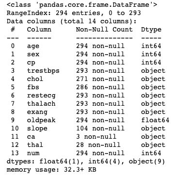
df.info()We can see here that columns 10, 11, and 12 have a lot of nulls. ‘ Ca’ and ‘thal’ are actually almost empty and ‘slope’ has only 104 entries. This is too many missing values to fill in so let’s drop them.
我们在这里可以看到第10、11和12列有很多空值。 “ Ca”和“ thal”实际上几乎是空的,“ slope”只有104个条目。 遗漏了太多的缺失值,因此我们将其删除。
df.drop(columns=['slope', 'thal', 'ca'], inplace=True)The rest of the columns have none or little missing values. For simplicity, I suggest dropping the entries that do have them. We should not lose too much data.
其余列没有缺失值或缺失值很小。 为简单起见,我建议删除包含它们的条目。 我们不应该丢失太多数据。
df.dropna(inplace=True)Another information that we could read from the result of the info() function is the fact that most of the columns are objects even though they seem to have numeric values.
我们可以从info()函数的结果中读取的另一个信息是,即使大多数列似乎都具有数字值,它们也是对象。
My suspicion is that this was caused by the question marks in the initial data set. Now that we have removed them we should be able to change the objects to numeric values.
我怀疑这是由初始数据集中的问号引起的。 现在我们已经删除了它们,我们应该能够将对象更改为数值。
In order to do this, we will use pd.to_numeric() function on the whole data frame. The object values should become numbers and it should not affect the values that already numbers.
为此,我们将在整个数据帧上使用pd.to_numeric()函数。 对象值应成为数字,并且不应影响已经为数字的值。
df = df.apply(pd.to_numeric)
df.info()
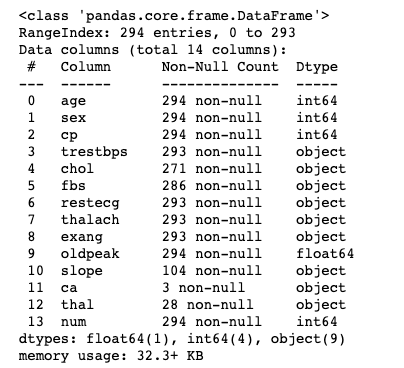
As you can see we are now left only with floats and integers. The info() function also confirm that the columns ‘ Ca’, ‘thal’, and ‘slope’ were dropped.
如您所见,我们现在只剩下浮点数和整数了。 info()函数还确认已删除列' Ca','thal'和'slope' 。
Also, rows with null values got removed and as a result, we have a data set with 261 numeric variables.
同样,具有空值的行也被删除,因此,我们有一个包含261个数字变量的数据集。
There is one more thing we need to do before we can proceed. I have noticed that the last column ‘num’ has some trailing spaces in its name (you cannot see this with a bare eye) so let’s have a look at the list of column names.
在继续之前,我们还需要做另一件事。 我注意到,最后一列“ num”的名称中有一些尾随空格(您不能用肉眼看到),因此让我们看一下列名称列表。
df.columnsYou should see the trailing spaces in the last column ‘num’. Let’s remove them by applying strip() function.
您应该在最后一列'num'中看到尾随空格。 让我们通过应用strip()函数将其删除。
df.columns = [column.strip() for column in df.columns]Done!
做完了!
Exploratory Data Analysis
探索性数据分析
Let’s do some basic data analysis. We are going to look at the distribution of variables using histograms first.
让我们做一些基本的数据分析。 我们将首先使用直方图查看变量的分布。
import matplotlib.pyplot as plt
plt.figure(figsize=(10,10))
df.hist()
plt.tight_layout()
What we can notice straight away is the fact that some variables are not continuous. Actually, only five features are continuous:’’age’, ‘chol’, ‘oldpeak’, ‘thalach’, ‘trestbps’ whereas the other are categorical variables.
我们可以立即注意到的事实是某些变量不是连续的。 实际上,只有五个特征是连续的:“ 年龄”,“胆汁”,“老峰”,“ thalach”,“ trestbps”,而另一个是分类变量。
Because we want to treat them differently in our exploration we should divide them into two groups.
因为我们希望在探索中区别对待它们,所以我们应将它们分为两组。
continous_features = ['age', 'chol', 'oldpeak', 'thalach', 'trestbps'] non_continous_features = list(set(df.columns) - set(continous_features + ['num']))After doing this you can check their values by typing the variable names in Jupyter notebook cell.
完成此操作后,您可以通过在Jupyter笔记本单元格中键入变量名称来检查其值。
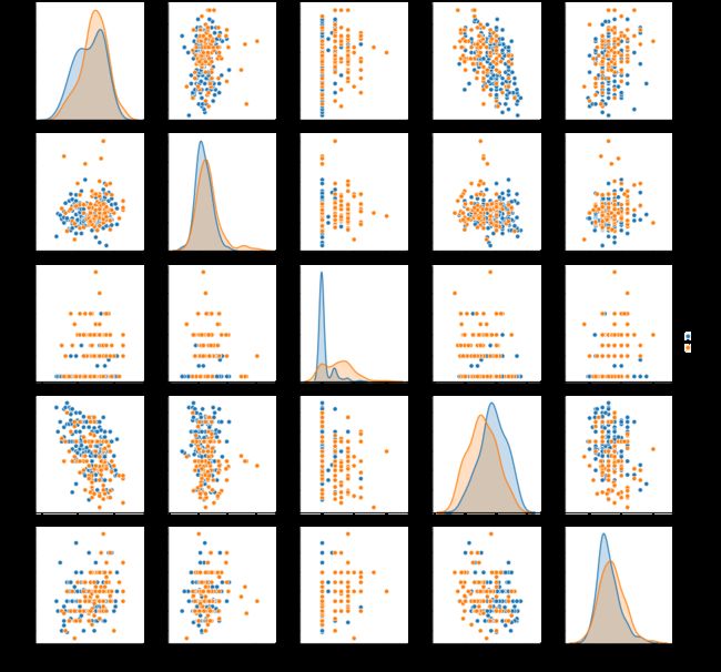
continous_featuresnon_continous_featuresNow we would like to inspect how the continuous features differ across the target variable. We will do this with a scatterplot.
现在,我们要检查连续特征在目标变量之间的差异。 我们将使用散点图进行此操作。
import seaborn as sns
df.num = df.num.map({0: 'no', 1: 'yes'})
sns.pairplot(df[continous_features + ['num']], hue='num')
* Note that we had to make the ‘num’ variable a string in order to use it as a hue parameter. We did it by mapping 0s to ‘no’ meaning healthy patients, and 1s to ‘yes’ meaning patients with heart disease.
*请注意,必须将'num'变量设置为字符串,才能将其用作色调参数。 我们通过将0映射到“ no”(表示健康患者),将1s映射到“ yes”(表示心脏病患者)来做到这一点。
If you look at the scatterplots and kdes you can see that there are district patterns for patients with heart disease in comparison to patients who are healthy.
如果您查看散点图和kdes,您会发现与健康患者相比,心脏病患者存在区域模式。
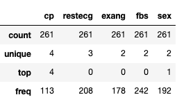
In order to explore categorical variables, we will look at distinct values they can take by using describe() function.
为了探索分类变量,我们将研究使用describe()函数可以获取的不同值。
df[non_continous_features].applymap(str).describe()We can see that ‘ exang’, ‘fbs’ and ‘sex’ are binary (they take only two distinct values). Whereas ‘cp’ and ‘resteceg’ take respectively four and three distinct values.
我们可以看到' exang','fbs'和'sex'是二进制的(它们仅采用两个不同的值)。 而“ cp”和“ resteceg”分别取四个和三个不同的值。
The last two are ordered categorical variables as encoded by the data set authors. I am not sure if we should treat them like that or change them to dummy encodings. This would need further investigation and we could change the approach in the future. For now, we will leave them ordered.
最后两个是由数据集作者编码的有序分类变量。 我不确定是否应该这样对待它们或将其更改为虚拟编码。 这需要进一步的调查,我们将来可能会改变方法。 目前,我们将让他们下订单。
Last but not least we are going to explore the target variable.
最后但并非最不重要的一点是,我们将探索目标变量。
df.num.value_counts()We have 163 healthy patients and 98 patients with heart problems. Not ideally balanced data set but that should be ok for our purposes.
我们有163名健康患者和98名心脏病患者。 不是理想的平衡数据集,但对于我们的目的应该是可以的。
Creating a baseline model
创建基准模型
After a quick exploratory data analysis, we are ready to build an initial classifier. We are going to start by dividing the data set into features and the target variable.
在快速探索性数据分析之后,我们准备构建初始分类器。 我们将从将数据集分为要素和目标变量开始。
X = df.drop(columns='num')
y = df.num.map({'no': 0, 'yes': 1})
* Note that I have to reverse the mapping I have applied while creating a seaborn graph, therefore, a need for map() function while creating y variable.
*请注意,在创建Seaborn图时,我必须反转我应用的映射,因此,在创建y变量时需要map()函数。
We also have used all features that the data set had as by looking at our quick EDA they all seemed relevant.
通过查看我们的快速EDA,我们还使用了数据集所具有的所有功能,它们似乎都很相关。
Now we will divide X and y variables further into their train and test correspondents using train_test_split() function.
现在,我们将使用train_test_split()函数将X和y变量进一步划分为它们的训练和测试对应项。
from sklearn.model_selection import train_test_splitX_train, X_test, y_train, y_test = train_test_split(X, y, test_size=0.2, random_state=1) X_train.shape, X_test.shape, y_train.shape, y_test.shapeAs a result of the above operations, we should have now four different variables: X_train, X_test, y_train, y_test whose dimensions are printed above.
作为上述操作的结果,我们现在应该具有四个不同的变量:X_train,X_test,y_train,y_test,其尺寸显示在上方。
Now we will build a baseline using a DummyClassifier.
现在,我们将使用DummyClassifier建立基线。
from sklearn.dummy import DummyClassifier
from sklearn.metrics import accuracy_score
dc = DummyClassifier(strategy='most_frequent')
dc.fit(X,y) dc_preds = dc.predict(X)
accuracy_score(y, dc_preds)
As you can see the baseline classifier is giving us 62% accuracy on the train set. The strategy for our baseline is predicting the most frequent class.
如您所见,基线分类器为我们提供了62%的火车准确率。 我们基线的策略是预测最频繁的课程。
Let’s see if we can beat it with Random Forest.
让我们看看是否可以用随机森林击败它。
Random Forest Classifier
随机森林分类器
The code below sets a Random Forest Classifier and uses cross-validation to see how well it performs on different folds.
下面的代码设置了一个随机森林分类器,并使用交叉验证来查看其在不同褶皱处的表现。
from sklearn.ensemble import RandomForestClassifier from sklearn.model_selection
import cross_val_score rfc = RandomForestClassifier(n_estimators=100, random_state=1)
cross_val_score(rfc, X, y, cv=5)
As you can see these accuracies are in general much higher than our dummy baseline. Only the last fold has lower accuracy. It looks like this last fold has examples that are hard to recognize.
如您所见,这些精度通常比我们的虚拟基准要高得多。 仅最后一折具有较低的准确性。 看起来这最后一折的例子很难辨认。
Nevertheless, if we take the average of those five, we get an accuracy of around 74%, and this is much higher than 62% baseline.
但是,如果我们取这五个平均值的平均值,则可以得到约74%的准确度,这比62%的基线要高得多。
Normally this is a stage where we would like to further tune model parameters using for example GridSearchCV but this is not a part of this tutorial.
通常,在这个阶段,我们希望使用例如GridSearchCV进一步调整模型参数,但这不是本教程的一部分。
Let’s see how well the model performs on the test set now. If you have paid attention we have not done anything with the test so far. It has been left alone until now.
让我们看看模型现在在测试集上的表现如何。 如果您已经注意,到目前为止,我们尚未对测试进行任何操作。 到现在为止,它一直被搁置。
Evaluating the model
评估模型
We will start by checking model performance in terms of accuracy.
我们将从检查模型性能的准确性开始。
First, we will fit the model using the whole training data, and then we will call the accuracy_score() function on the test parts.
首先,我们将使用整个训练数据拟合模型,然后在测试零件上调用precision_score()函数。
rfc.fit(X_train, y_train)
accuracy_score(rfc.predict(X_test), y_test)
We are getting 75% accuracy on the test. Similar to our average cross-validation accuracy calculation on the train set which was 74%.
我们在测试中获得75%的准确性。 与我们在火车上的平均交叉验证准确性计算相似,为74%。
Let’s see how well the Dummy classifier does on the test set.
让我们看看虚拟分类器在测试集上的表现如何。
accuracy_score(dc.predict(X_test), y_test)Accuracy for the baseline classifier is around 51%. This is actually much worse than the accuracy of our random forest model.
基线分类器的准确性约为51%。 这实际上比我们的随机森林模型的准确性差得多。
However, we should not only look at accuracy when evaluating a classifier. Let’s have a looks at confusion matrices for both random forest and the baseline model.
但是,我们不仅应该在评估分类器时考虑准确性。 让我们看一下随机森林和基准模型的混淆矩阵。
We will start with computing confusion matrix for Random Forest using scikit-learn function.
我们将从使用scikit-learn函数为随机森林计算混淆矩阵开始。
from sklearn.metrics import plot_confusion_matrix
plot_confusion_matrix(rfc, X_test, y_test)
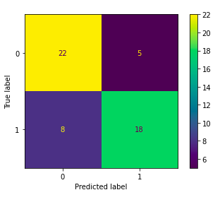
Actually we are not doing bad at all. We only have five False Positives, and also eight False Negatives. Additionally, we have predicted heart disease for eighteen people out of twenty-six people that had heart problems.
实际上,我们一点都没有做坏。 我们只有五个假阳性,还有八个假阴性。 此外,我们已经预测出26位患有心脏疾病的人中有18位患有心脏病。
Not great but not that bad. Note that we did not even tune the model!
不是很好,但不是那么糟糕。 请注意,我们甚至都没有调整模型!
Let’s compare this confusion matrix with the one calculated for the baseline model.
让我们将这个混淆矩阵与为基线模型计算出的混淆矩阵进行比较。
from sklearn.metrics import plot_confusion_matrix
plot_confusion_matrix(dc, X_test, y_test)
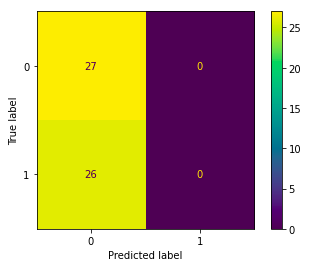
Have a closer look at the graph above. Can you see that we always predict label 0? This means we predict that all patients are healthy!
请仔细查看上图。 您看到我们总是预测标签0吗? 这意味着我们可以预测所有患者都健康!
That is right, we have set our Dummy Classifier to predict the majority class. Note that it would be a terrible model for our purposes as we would not discover any patients with heart issues.
没错,我们已经将虚拟分类器设置为预测多数分类。 请注意,对于我们的目的,这将是一个糟糕的模型,因为我们不会发现任何有心脏问题的患者。
Random Forest did much better! We actually have discovered 18 people with heart problems out of 26 in the test set.
随机森林好多了! 实际上,在测试集中的26名患者中,我们发现了18名患有心脏疾病的人。
Summary
摘要
In this post, you have learned how to build a basic classifier using Random Forest.
在本文中,您学习了如何使用随机森林构建基本分类器。
It was rather an overview of the main techniques that are used when building a model on a data set without going into too many details.
它只是对在数据集上构建模型时使用的主要技术的概述,而无需涉及太多细节。
This was intended so this article does not get too long and serves as a starting point for someone who wants to build their first classifier.
这样做的目的是使本文不会太长,并且可以作为想要构建其第一个分类器的人的起点。
Happy Learning!
学习愉快!
Originally published at https://www.aboutdatablog.com on August 13, 2020.
最初于 2020年8月13日 发布在 https://www.aboutdatablog.com 。
PS: I am writing articles that explain basic Data Science concepts in a simple and comprehensible on aboutdatablog.com. If you liked this article there are some other ones you may enjoy:
PS:我写的文章在 aboutdatablog.com 上以简单易懂的方式解释了基本的数据科学概念 。 如果您喜欢这篇文章,您可能还会喜欢其他一些文章:
翻译自: https://towardsdatascience.com/build-your-first-random-forest-classifier-cbc63a956158
随机森林分类器

