第二讲-神经网络优化-损失函数
5、损失函数
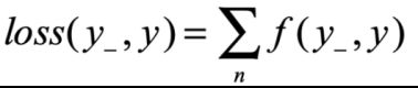
损失函数是前向传播计算出的结果y与已知标准答案y_的差距。神经网络的优化目标,找出参数使得loss值最小。
本次介绍损失函数有:均方误差(mse,Mean Squared Error)、自定义、交叉熵(ce,Cross Entropy)
- 均方误差( y_表示标准答案,y表示预测答案计算值)

tensorFlow : lose_mse =tf.reduce_mean(tf.square(y-y’))
示例:预测酸奶日销量y,x1,x2是影响因素。建模前,应预先采集数据:每日x1,x2和销量y_。拟造数据集X,Y_:y_=x1+x2 噪声:-0.05~+0.05.
代码:
import tensorflow as tf
import numpy as np
SEED = 23455
rdm = np.random.RandomState(seed=SEED) # 生成[0,1)之间的随机数
x = rdm.rand(32,2) # 随机制造训练数据x和 y_
y_ = [[x1 + x2 + (rdm.rand()/10.0-0.05)] for (x1,x2) in x] # 生成噪声[0,1)/10=[0,0.1); [0,0.1)-0.05=[-0.05,0.05)
x = tf.cast(x,dtype=tf.float32)
w1 = tf.Variable(tf.random.normal([2,1],stddev=1,seed=1))
epoch = 15000
lr = 0.002
for epoch in range(epoch):
with tf.GradientTape() as tape:
y = tf.matmul(x,w1)
loss_mse = tf.reduce_mean(tf.square(y_ - y))
grads = tape.gradient(loss_mse,w1)
w1.assign_sub(lr * grads)
if(epoch % 500==0):
print("After %d training steps,w1 is " % (epoch))
print(w1.numpy(),'\n')
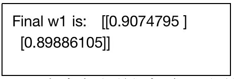
print("Final w1 is: ", w1.numpy())
运行结果:
After 0 training steps,w1 is
[[-0.8096241]
[ 1.4855157]]
After 500 training steps,w1 is
[[-0.21934733]
[ 1.6984866 ]]
After 1000 training steps,w1 is
[[0.0893971]
[1.673225 ]]
。。。。
After 14000 training steps,w1 is
[[0.9993659]
[0.999166 ]]
After 14500 training steps,w1 is
[[1.0002553 ]
[0.99838644]]
Final w1 is: [[1.0009792]
[0.9977485]]最终W1均接近1,预测符合预期。
如预测商品销量,预测多了,损失成本;预测少了,损失利润。如果利润!=成本,因mse会同等对待各个因素,则mse产生的loss无法利益最大化。从而可以根据实际情况进行自定义损失函数。
损失函数的定义能极大影响预测效果。好的损失函数设计对于模型训练能起到良好的引导作用。
- 自定义损失函数
同样以预测酸奶销量为例:自定义损失函数为:

loss_zdy=tf.reduce_sum(tf.where(tf.greater(y,y_),(y-y_)*COST,(y_-y)*PROFIT))
如酸奶成本(COST)1元,利润(PROFIT)99元。预测少了损失利润99元,大于预测多了损失成本1元。预测少了损失大,希望生成的预测函数往多了预测。
完整代码(相比mse代码,仅修改了 # ----):
import tensorflow as tf
import numpy as np

SEED = 23455
COST = 1    #  ----
PROFIT = 99     # ----

rdm = np.random.RandomState(seed=SEED)      # 生成[0,1)之间的随机数
x = rdm.rand(32,2)     # 随机制造训练数据x和 y_
y_ = [[x1 + x2 + (rdm.rand()/10.0-0.05)] for (x1,x2) in x]    # 生成噪声[0,1)/10=[0,0.1); [0,0.1)-0.05=[-0.05,0.05)
x = tf.cast(x,dtype=tf.float32)

w1 = tf.Variable(tf.random.normal([2,1],stddev=1,seed=1))

epoch = 15000
lr = 0.002

for epoch in range(epoch):
    with tf.GradientTape() as tape:
        y = tf.matmul(x,w1)
        loss_zdy = tf.reduce_sum(tf.where(tf.greater(y,y_),(y-y_)*COST,(y_-y)*PROFIT))     # ----

    grads = tape.gradient(loss_zdy,w1)
    w1.assign_sub(lr * grads)

    if(epoch % 500==0):
        print("After %d training steps,w1 is " % (epoch))
        print(w1.numpy(),'\n')
print("Final w1 is: ", w1.numpy())


运行结果:
。。。
Final w1 is:  [[1.1420636]
 [1.1016785]]
查看运行最终w1,可见参数均大于1,预测均偏多。
若修改COST=99, PROFIT =1,再次运行查看final w1:
可见,当成本比利润高时,预测的w均小于1,预测量偏少。
- 交叉熵损失函数(Cross Entropy)
表征两个概率分布之间的距离。
交叉熵越大,两个概率分布越远;
交叉熵越小,两个概率分布越近。
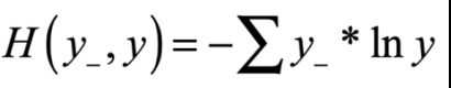
tensorFlow: tf.losses.categorical_crossentropy(y_,y)
例如:二分类已知答案y_=(1,0),预测y1=(0.6,0.4),y2=(0.8,0.2),哪个更接近标准答案?
代码计算:
import tensorflow as tf
loss_ce1 = tf.losses.categorical_crossentropy([1,0],[0.6,0.4])
loss_ce2 = tf.losses.categorical_crossentropy([1,0],[0.8,0.2])
print("loss_ce1:",loss_ce1)
print("loss_ce2:",loss_ce2)

运行结果:
loss_ce1: tf.Tensor(0.5108256, shape=(), dtype=float32)
loss_ce2: tf.Tensor(0.22314353, shape=(), dtype=float32)
因为loss_ce1>loss_ce2,故y2预测更准确。
- softmax与交叉熵结合
输出先过softmax函数,再计算y与y-的交叉熵损失函数。
tf.nn.softmax_cross_entropy_with_logits(y_,y) --同时计算了softmax和交叉熵
示例:
import tensorflow as tf
import numpy as np

y_ = np.array([[1, 0, 0], [0, 1, 0], [0, 0, 1], [1, 0, 0], [0, 1, 0]])
y = np.array([[12, 3, 2], [3, 10, 1], [1, 2, 5], [4, 6.5, 1.2], [3, 6, 1]])
y_pro = tf.nn.softmax(y)
loss_ce1 = tf.losses.categorical_crossentropy(y_,y_pro)
loss_ce2 = tf.nn.softmax_cross_entropy_with_logits(y_, y)

print('分步计算的结果:\n', loss_ce1)
print('结合计算的结果:\n', loss_ce2)

运行结果:
分步计算的结果:
 tf.Tensor(
[1.68795487e-04 1.03475622e-03 6.58839038e-02 2.58349207e+00
 5.49852354e-02], shape=(5,), dtype=float64)
结合计算的结果:
 tf.Tensor(
[1.68795487e-04 1.03475622e-03 6.58839038e-02 2.58349207e+00
 5.49852354e-02], shape=(5,), dtype=float64)
可见,loss_ce2 一行代码等同于 y_pro, loss_ce1,2行代码效果。