r语言 支持向量机实现_支持向量机解密：R中的实现

r语言 支持向量机实现

Support Vector Machine, popularly abbreviated as SVM is a supervised learning algorithm used for both regression and classification but more commonly used for classification. SVMs have been shown to outperform well in a variety of setting and are often considered as one of the best “out of box” classifiers.

支持向量机(Support Vector Machine)，通常缩写为SVM，是一种用于回归和分类的监督学习算法，但更常用于分类。 SVM在各种设置下均表现出色，通常被认为是最好的“开箱即用”分类器。

In this article we will discuss SVMs for a 2-class classification setting. The approach used in Support Vector Machines is based on finding a separting hyperplane.

在本文中，我们将讨论用于2类分类设置的SVM。 支持向量机中使用的方法是基于找到分离的超平面 。

Let us start by defining a hyperplane.

让我们首先定义一个超平面。

什么是超平面？ (What is a hyperplane?)

In a p dimensional space, a hyperplane(H) is a flat affine subspace of dimension p-1. In other words, if V is a p-dimensional vector space than H is a (p-1) dimensional subspace. Examples of hyperplanes in 2 dimensions are any straight line through the origin. In 3 dimensions, any plane containing the origin.

在ap维空间中，超平面(H)是维p-1的平仿射子空间。 换句话说，如果V是p维向量空间，则H是(p-1)维子空间。 二维超平面的示例是通过原点的任何直线。 在3维中，包含原点的任何平面。

a point X 点X

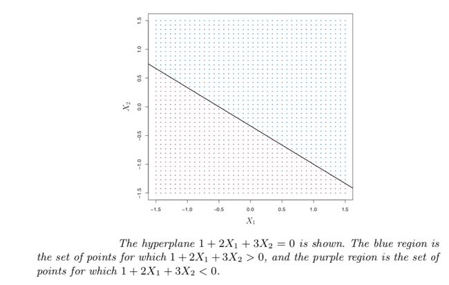
The hyperplane mentioned above divides the p-dimensional space into two halves. Depending on whether the equation is >0 or <0 , the point X lies on either sides of the hyperplane.

上述超平面将p维空间分为两半。 根据等式是> 0还是<0，点X位于超平面的两侧。

Figure 1 图1

使用分离的超平面进行分类 (Classification Using a Separating Hyperplane)

Now that we have understood what a hyperplane is, let us take another step forward towards building a classifier based on a separating hyperplane. If such a hyperplane exists which can separate our training observations into two classes namely y_i=1 and y_i=-1 then the hyperplane has the following properties;

既然我们已经了解了什么是超平面，那么让我们朝着基于分离的超平面构建分类器又迈出一步。 如果存在这样的超平面，可以将我们的训练观察结果分为两类，即y_i = 1和y_i = -1，则该超平面具有以下属性；

De facto, this can be written in one single equation as;

实际上，这可以写成一个方程：

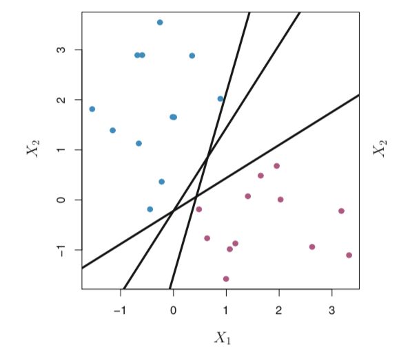
for all i=1,2,…,n 对于所有i = 1,2，…，n

There could be infinite number of such hyperplanes. The figure below shows three such hyperplanes;

这样的超平面可能是无限的。 下图显示了三个这样的超平面；

Figure 2 : solid lines represent 3 separating hyperplanes which separate the training observations into two classes; blue and purple. 图2：实线表示3个分离的超平面，它们将训练观察结果分为两类； 蓝色和紫色。

If a separating hyperplane exists, we can use it to construct a very trivial classifier : a test observation(x) is assigned a class depending on which side of the hyperplane it is located(by looking at the sign of the above equation) . We can also make use of the magnitude of the equation of the hyperplane. If it is large, x lies far away from the hyperplane so we can be more confident about our class assignment for x.

如果存在分离的超平面，我们可以使用它构造一个非常简单的分类器：根据测试观测值(x)所在的超平面的哪一侧为其分配一个类(通过查看上述方程式的符号)。 我们还可以利用超平面方程的大小。 如果它很大，则x远离超平面，因此我们可以更自信地分配x的类。

The question now is, is there a way to decide which of these infinite hyperplanes should we use? To tackle this, comes in the Maximal Margin Classifier.

现在的问题是， 有没有办法确定我们应该使用这些无限超平面中的哪一个？ 为了解决这个问题，请使用“ 最大保证金分类器”。

最大保证金分类器 (The Maximal Margin Classifier)

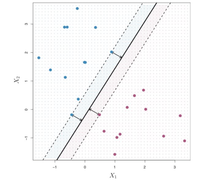
This is also known as the optimal separating hyperplane which is the hyperplane that is farthest from the training observation . We obtain this by calculating the perpendicular distance from each training observation to the hyperplane. The smallest of these distances is the minimum distance of the hyperplane from the training observations and is known as the margin. The maximal margin hyperplane is the hyperplane for which this margin is the largest. Now we can easily classify our test observation depending on which side of the maximal margin hyperplane does it lie. This is known as the Maximal Margin Classifier.

这也称为最佳分离超平面，它是距离训练观测值最远的超平面。 我们通过计算从每个训练观测值到超平面的垂直距离来获得此距离 。 这些距离中的最小距离是超平面距训练观测值的最小距离，称为边距。 最大余量超平面是该余量最大的超平面。 现在，我们可以根据最大观察值超平面位于哪一侧轻松地对测试观察结果进行分类。 这称为最大保证金分类器。

Remember, if p is large, the maximal margin classifier could also lead to overfiiting.

请记住，如果p大，则最大余量分类器也可能导致过拟合。

Figure 3: The solid line is the separating hyperplane and the dashed line represents the margin. 图3：实线是分隔的超平面，虚线表示边距。

In figure 3, there are 3 observations which lie on the dashed line(margin). These observations are known as “support vectors” since they support the maximal margin hyperplane in a sense that if they move even slightly the hyperplane would move as well.

在图3中，虚线(边距)上有3个观测值。 这些观测值被称为“支持向量”，因为它们在某种意义上支持最大余量超平面，即使它们稍微移动，超平面也将移动。

Note: The maximal margin hyperplane depends directly only on the movement of these support vectors but not on the movement of the other observations provided they do not move to the other side of the separating hyperplane.

注意：最大余量超平面仅直接取决于这些支持向量的运动，而不取决于其他观测值的运动，只要它们不移至分离超平面的另一侧即可。

The optimization problem of finding the maximal margin hyperplane can be written mathematically as;

找到最大余量超平面的优化问题可以用数学写成：

Here, M represents the margin of the hyperplane and the optimization problem chooses ßs which maximize M. Actually, for each observation to be on the correct side of the hyperplane we would require the 2nd constraint to be >0 but we want the observation to be on the right side of the margin as well and hence we require it to be ≥M. This constraint guarantees each observation will be on the correct side, provided M is positive.

在此，M代表超平面的余量，优化问题选择使M最大化的ßs。实际上，对于每个观测值都在超平面的正确侧，我们将要求第二约束> 0，但我们希望观测值是同样在边距的右侧，因此我们要求它≥M。 如果M为正，则此约束条件可确保每个观察值都在正确的一侧。

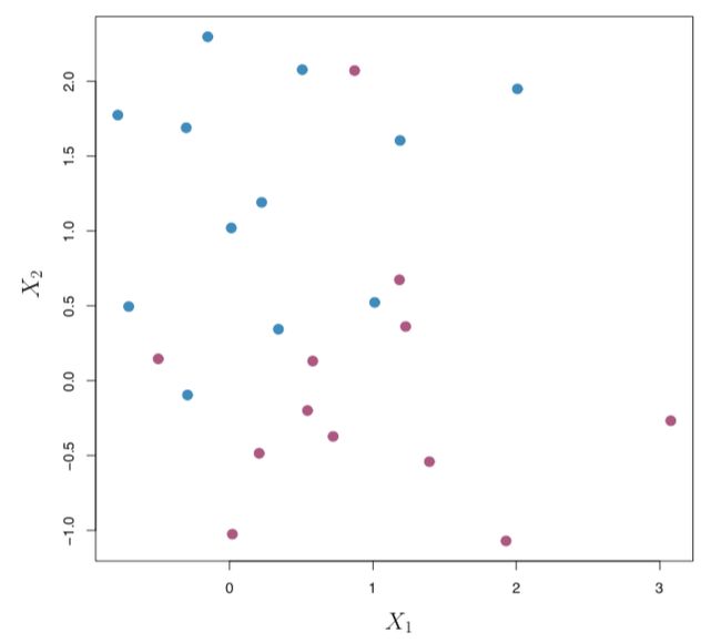
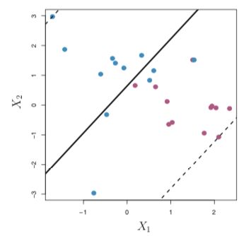
The maximal margin classifier is a very natural approach if a separating hyperplane exists. However, in many cases no separating hyperplane exists, and so there is no maximal margin classifier. In this case, the above optimization problem has no solution with M > 0. As you can see in Figure 4 below, we cannot exactly separate observations into two classes. For scenarios like these, we can find a hyperplane that “almost” separates the classes.

如果存在分离的超平面，则最大余量分类器是非常自然的方法。 但是，在许多情况下，不存在分离的超平面，因此不存在最大余量分类器。 在这种情况下，上面的优化问题无法解决M> 0的问题。如下面的图4所示，我们无法将观察结果精确地分为两类。 对于此类情况，我们可以找到一个“ 几乎”将各类分开的超平面。

Figure 4 图4

This generalization of the maximal margin classifier to a non-separable case is called support vector classifier. This is often known as the soft margin classifier as well.

最大余量分类器到不可分情况的这种概括被称为支持向量分类器。 这通常也称为软边距分类器。

支持向量分类器 (The Support Vector Classifier)

Developing a classifier that almost separates classes is done by the soft margin formula. Sometimes, it might be the case that by adding just one observation more, the hyperplane changes drastically. This indicates, the hyperplane might have overfitted our training data. In these cases, it would we worthwhile to miss-classify a certain number of observations so that the remaining observations are classified more accurately. We allow some observations to be on the incorrect side of the margin, or even on the incorrect side of the hyperplane. This is the soft margin formula, and the word soft refers to the fact that the margin can be violated by a fixed number of training observations.

开发几乎将类分离的分类器是通过软边距公式完成的。 有时，可能情况可能是，仅增加一个观测值，超平面就会急剧变化。 这表明，超飞机可能过度拟合了我们的训练数据。 在这些情况下，我们值得对某些观测值进行误分类，以便对其余观测值进行更准确的分类。 我们允许某些观测值位于边界的不正确的一侧，甚至位于超平面的不正确的一侧。 这是软保证金公式，“ 软 ”一词指的是一定数量的训练观测值可能违反保证金的事实。

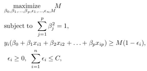
The classification rule is to classify a test observation depending on which side of a hyperplane it lies. The hyperplane is chosen so that it correctly classifies most of the training observations, but may misclassify a few observations. It is the solution to the optimization problem:

分类规则是根据其位于超平面的哪一侧对测试观察进行分类。 选择超平面，以便它可以正确分类大多数训练观测值，但可能会误分类一些观测值。 它是优化问题的解决方案：

C is a non-negative tuning parameter C是非负调整参数

M is the width of the margin and we seek to make this quantity as large as possible. ε_1, . . . , ε_n are known as slack variables which tell us where each observation lies. If ε_i=0 the ith observation is on the correct side of the margin. If εi > 0 then the ith observation is on the wrong side of the margin. If εi > 1 then it is on the wrong side of the hyperplane. As in the earlier sections, we classify the obserervations to a particular class based on the sign of;

M是边距的宽度，我们试图使此数量尽可能大。 ε_1，。 。 。 ，ε_n被称为松弛变量 ，它告诉我们每个观察值在哪里。 如果ε_i= 0，则第i个观测值位于边界的正确一侧。 如果εi> 0，则第i个观测值位于边界的错误一侧。 如果εi> 1，则它在超平面的错误一侧。 与前面的部分一样，我们根据的符号将观察到的事物分类为特定的类。

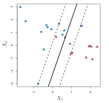
Let us now discuss the tuning parameter C in more detail. C puts an upper bound to the sum of ε_i’s, and hence determines the number of violations to the margin and hyperplane which are allowed. If C = 0 then there is no scope for violations and ε1 = … = εn = 0, in which case this simply becomes a maximal margin hyperplane optimization problem. If C>0, no more than C observations can be on the wrong side of the hyperplane (because then ε_i > 1 and we require ∑ε_i≤C). As C increases, we allow more violations to the margin, and so the margin will widen and vice versa.

现在让我们更详细地讨论调整参数C。 C将ε_i的总和作为上限，因此确定了允许的违反边距和超平面的次数。 如果C = 0，则不存在违反范围，并且ε1=…=εn= 0，在这种情况下，这仅成为最大余量超平面优化问题。 如果C> 0，则在超平面的错误一侧最多可以有C个观测值(因为ε_i> 1并且我们要求∑ε_i≤C)。 随着C的增加，我们允许更多的违反行为，因此，保证金将会扩大，反之亦然。

Only the observations that either lie on the margin or that violate the margin will affect the hyperplane. Observations that lie directly on the margin, or on the wrong side of the margin, are known as support vectors. The observations that lies strictly on the correct side of the margin do not affect the support vector classifier.

只有位于边缘或违反边缘的观测值才会影响超平面。 直接位于边缘或边缘错误一侧的观测值称为支持向量 。 严格位于边距正确侧的观察结果不会影响支持向量分类器。

Figure 5: A large value of C results in a wider margin 图5：较大的C值导致较宽的余量

Figure 6: A smaller value of C results in a less wider margin 图6：较小的C值导致较小的边距

The support vector classifier is a natural approach for classification if the boundary between the two classes is linear. However, in real life situations we are sometimes faced with non-linear class boundaries.

如果两个类别之间的边界是线性的，则支持向量分类器是一种自然的分类方法。 但是，在现实生活中，我们有时会面临非线性的阶级界限。

Figure 7 : A linear boundary performs poorly on this dataset as it cannot be separated by a linear boundary 图7：线性边界在此数据集上的表现较差，因为它不能被线性边界分开

One way to tackle this problem is to consider enlarging the feature space using functions of the predictor variables ,such as quadratic and cubic terms, which will help us address this non-linearity. However, there are many possible functions we could add and we could end up with a huge number of features which become computationally unmanageable.

解决此问题的一种方法是考虑使用预测变量的函数(例如二次项和三次项)扩大特征空间，这将有助于我们解决此非线性问题。 但是，我们可以添加许多可能的功能，最终可能会产生大量功能，这些功能在计算上变得难以管理。

To improve upon this problem we introduce the Support Vector Machine which allows us to enlarge the feature space in a way that leads to efficient computations.

为了改善这个问题，我们引入了支持向量机 ，它使我们能够以导致高效计算的方式扩大特征空间。

支持向量机(SVM) (The Support Vector Machine (SVM))

SVM is further an extension of the support vector classifier that results from enlarging the feature space in a specific way, using “kernels”. When the support vector classifier is combined with a non-linear kernel, the resulting classifier is known as a support vector machine.

SVM是支持向量分类器的进一步扩展，它是通过使用“ 内核 ”以特定方式扩大特征空间而产生的。 当支持向量分类器与非线性内核组合时，所得分类器称为支持向量机。

A kernel is a function that quantifies the similarity of two observations. It is represented as;

核是一种量化两个观测值相似性的函数。 它表示为；

K is a function known as kernel K是一个称为内核的函数

For instance, the kernel shown here is a Linear Kernel ;

例如，这里显示的内核是线性内核 ；

The kernel is linear here because the support vector classifier is linear in the features. This is also commonly known as the dot product.

这里的核是线性的，因为支持向量分类器在特征上是线性的。 这也通常称为点积。

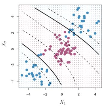
Other kernels can also be used that transform the input space into higher dimensions such as Polynomial Kernel or Radial Kernel. This is popularly known as the Kernel Trick.

也可以使用其他将输入空间转换成更高维度的内核，例如多项式内核或径向内核 。 这是众所周知的内核技巧。

Polynomial Kernel:

多项式内核：

This is known as a polynomial kernel of degree d. This amounts to fitting a support vector classifier in a higher-dimensional space involving polynomials of degree d, rather than in the original space which leads to a much more flexible decision boundary. If d=1 in the above equation, it reduces to a support vector classifier seen earlier.

这被称为度d的多项式核。 这等于将支持向量分类器拟合到包含次数为d的多项式的高维空间中，而不是在原始空间中拟合，从而导致决策边界更加灵活。 如果上式中的d = 1，则将其简化为较早见到的支持向量分类器。

Radial Kernel:

径向内核：

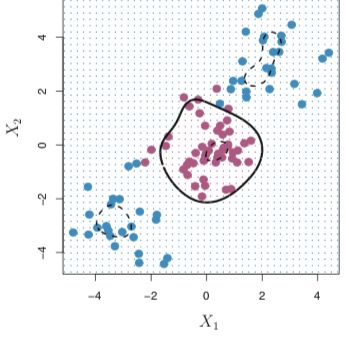
Here, γ is a positive constant. In case of a radial kernel, if a test observation (x) is far from a training observation x_i then the summation term in the above expression is large and so the kernel function will be very small. So, this particular training observation will play no role in predicting the class for test observation x. More generally, training observations that are far from x will essentially play no role in predicting the class label for x.

在此，γ为正常数。 在径向核的情况下，如果测试观测值(x)与训练观测值x_i相距甚远，则上述表达式中的总和项将很大，因此核函数将非常小。 因此，这种特定的训练观察将不会在预测测试观察x的类别中发挥任何作用。 更一般而言，远离x的训练观测值在预测x的类别标签上基本上不起作用。

Figure 8: SVM with a polynomial kernel 图8：具有多项式内核的SVM

Figure 9: SVM with a radial kernel 图9：具有径向内核的SVM

在R中执行 (Implementation in R)

Let us start by generating some 2 dimensional data and make them a little separated. Construct a matrix x with 20 observations in 2 classes on 2 variables. Then construct a y variable, which will be -1 or 1, with 10 in each class. Plotting the data will help you visualise the dataset having two classes-red and blue.

让我们首先生成一些二维数据，并将它们分开一些。 使用2个变量的2个类构造具有20个观测值的矩阵x 。 然后构造一个y变量，该变量将为-1或1，每个类中有10个。 绘制数据有助于您可视化具有红色和蓝色两个类别的数据集。

set.seed(10111) 
x=matrix(rnorm(40), 20, 2) 
y=rep(c(-1, 1), c(10, 10)) 
x[y==1,]=x[y==1,] + 1 
plot(x,col=y + 3,pch=19)

We will use the svm() function in the library “e1071”. We make a dataframe of the data and encode the y variable as a factor variable. The argument scale=FALSE tells the svm() function not to scale each feature to have mean zero or standard deviation one.

我们将在库“ e1071”中使用svm()函数。 我们创建数据的数据框，并将y变量编码为因子变量。 参数scale = FALSE告诉svm()函数不要将每个特征缩放为均值为零或标准差为1。

dat=data.frame(x,y=as.factor(y))
library(e1071)
svmfit=svm(y ~ .,data=dat,kernel="linear",cost=10,scale=FALSE)
print(svmfit)
plot(svmfit,dat)

Printing the svmfit gives its summary. You can see that the number of support vectors is 6 (the points that are close to the boundary or on the wrong side of the boundary). There’s a plot function for SVM that shows the decision boundary, as shown below;

打印svmfit给出其摘要。 您可以看到支持向量的数量为6(靠近边界或边界错误侧的点)。 SVM有一个绘图函数，它显示决策边界，如下所示；

You can now try to implement SVM in R using different kernels by varying the kernel parameter in the svm() function.

现在，您可以通过更改svm()函数中的内核参数，尝试使用不同的内核在R中实现SVM。

结论与参考 (Conclusion and References)

Support vector machine is a powerful algorithm and offers great accuracy and work well with high dimensional spaces.

支持向量机是一种功能强大的算法，具有很高的准确性，并且可以在高维空间中很好地工作。

References used;

使用的参考；

• An Introduction to Statistical Learning: with Applications in R
  统计学习入门：在R中的应用
• The Elements of Statistical Learning: Data Mining, Inference, and Prediction
  统计学习的要素：数据挖掘，推理和预测
• All figures are taken from ISLR
  所有数字均取自ISLR

• https://machinelearningmastery.com/support-vector-machines-for-machine-learning/

  https://machinelearningmastery.com/support-vector-machines-for-machine-learning/

• https://en.wikipedia.org/wiki/Support_vector_machine

  https://zh.wikipedia.org/wiki/Support_vector_machine

• https://scikit-learn.org/stable/modules/svm.html

  https://scikit-learn.org/stable/modules/svm.html

Thank you.

谢谢。

翻译自: https://medium.com/snu-ai/demystifying-support-vector-machines-with-implementations-in-r-9c5289a29e12

r语言 支持向量机实现