Lecture 4_Extra Graph Neural Networks
Lecture 4_Extra Graph Neural Networks
文章目录
- GNN
-
- Introduction
-
- Neural Network
- CNN
- RNN
- Transformer
- Graph
- GNN
-
- Why do we need GNN?
-
- Classification
- Generation
- Example
- How to train a GNN?
-
- Think about Convolution
- GNN Roadmap
- Tasks, Dataset, and Benchmark
-
- Tasks
- Common Datasets
- Benchmark
-
- Graph Classification: SuperPixel MNIST and CIFAR10
- Regression: ZINC molecule graphs dataset
- Node classification: Stochastic Block Model dataset
- Edge classification: Traveling Salesman Problem
- Results
-
- SuperPixel
- Regression
- Stochastic Block Model dataset
- Traveling Salesman Problem
- Spatial-based GNN
-
- Review: Convolution
- Spatial-based Convolution
- NN4G (Neural Networks for Graph)
- DCNN (Diffusion-Convolution Neural Network)
- DGC (Diffusion Graph Convolution)
- MoNET (Mixture Model Networks)
- GraphSAGE
- GAT (Graph Attention Networks)
- GIN (Graph Isomorphism Network)
- Graph Signal Processing and Spectral-based GNN
-
- Spectral-based CNN
- Spectral Graph Theory
-
- Example
-
- Vertex domain signal
- Filtering
- ChebNet
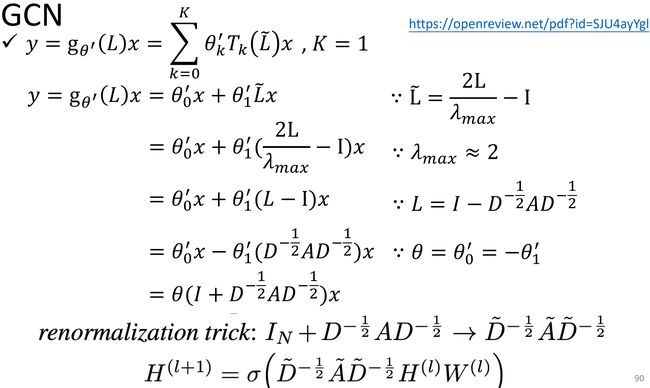
- GCN
GNN
Introduction
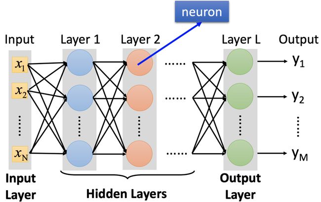
Neural Network
CNN
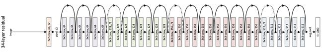
https://arxiv.org/pdf/1512.03385.pdf
RNN

Transformer
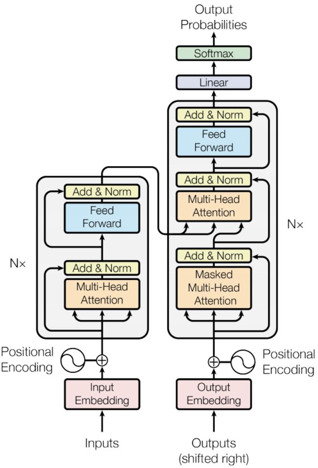
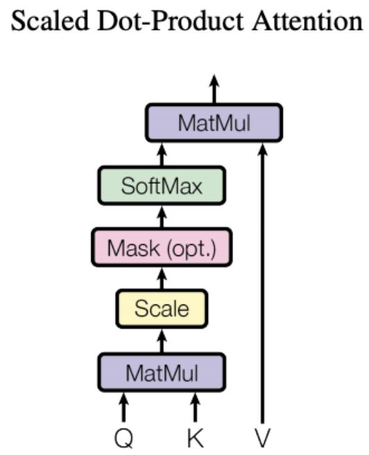
https://arxiv.org/pdf/1706.03762.pdf
http://speech.ee.ntu.edu.tw/~tlkagk/courses/ML_2019/Lecture/Transformer%20(v5).pdf
Graph
GNN
Why do we need GNN?
Classification
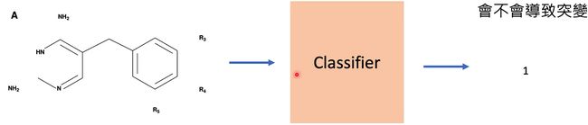
https://persagen.com/files/misc/scarselli2009graph.pdf
训练一个分类器,来识别某一分子是否会导致突变。
Generation
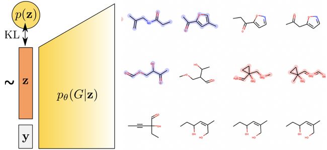
GraphVAE: https://arxiv.org/pdf/1802.03480.pdf
生成新药物的分子。
- How do we utilize the structures and relationship to help our model?
- What if the graph is larger, like 20k nodes?
- What if we don’t have the all the labels?
Example
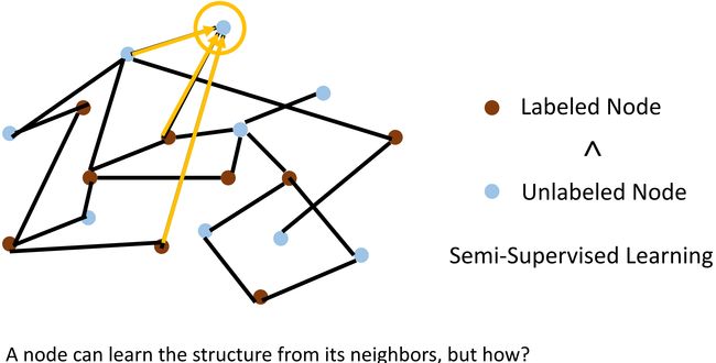
如上图所示,图中有两种 Node,在一些场景中,Unlabeled Node 的数量远大于 Labeled Node。在这种情况下,如何利用少数的 Labeled Node 以及周围邻居 structure 信息做一个好的 Node Representation,来训练从好的模型呢?
How to train a GNN?
Think about Convolution
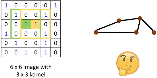
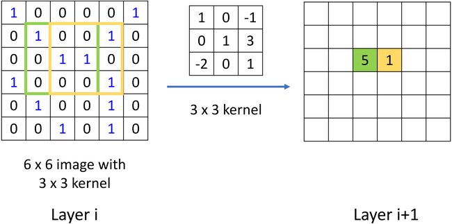
如上左图所示,对于绿色和黄色区域,我们可以用 k e r n e l kernel kernel 去做相乘再相加的卷积操作,从而得到下一层的 feature map \text{feature map} feature map。如何把这种操作泛化到 graph 呢?也就是,也能够在 graph 上做相乘相加,再 weighted sum \text{weighted sum} weighted sum 来完成一个类似的 “卷积” 操作。—— 好像不太容易。
- How to embed node into a feature space using convolution?
- Solution 1: Generalize the concept of convolution (co-relation) to graph >> Spatial-based convolution
- Solution 2: Back to the definition of convolution in signal processing >> Spectral-based convolution
GNN Roadmap

Tasks, Dataset, and Benchmark
Tasks
- Semi-supervised node classification
- Regression
- Graph classification
- Graph representation learning
- Link prediction
Common Datasets
- CORA: citation network. 2.7k nodes and 5.4k links
- TU-MUTAG: 188 molecules with 18 nodes on average
Benchmark
Graph Classification: SuperPixel MNIST and CIFAR10
Regression: ZINC molecule graphs dataset
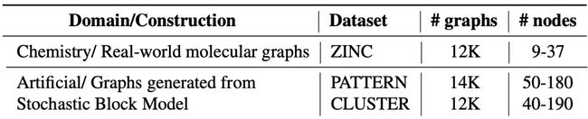
Node classification: Stochastic Block Model dataset
1711.07553.pdf (arxiv.org)

Edge classification: Traveling Salesman Problem
Results
SuperPixel

Regression
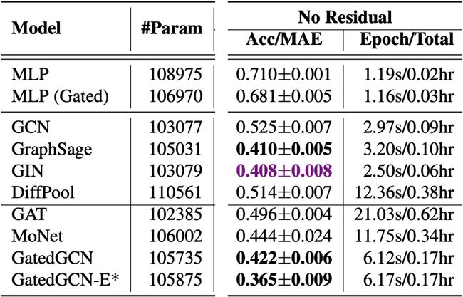
Stochastic Block Model dataset
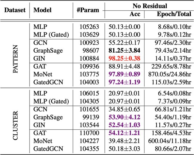
Traveling Salesman Problem


Spatial-based GNN
Review: Convolution
Spatial-based Convolution
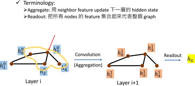
假设 input graph 如上左图所示,图中每个 node 都有一个 hidden feature h i 0 h_i^0 hi0。我们希望通过一个 c o n v o l u t i o n convolution convolution 操作来得到下一层各个 node 的 hidden feature h i 1 h_i^1 hi1。以 h 3 h_3 h3 为例介绍这一过程, h 3 0 h_3^0 h30 有 3 3 3 个邻居 h 0 0 , h 2 0 , h 4 0 h_0^0,\ h_2^0,\ h_4^0 h00, h20, h40, h 3 1 h_3^1 h31 将由这 3 3 3 个邻居间的计算得到,这一过程叫做 a g g r e g a t i o n aggregation aggregation,也就是利用邻居的 hidden feature 来得到下一层的 hidden state。
有时候我们需要得到一整个图的表示(而不是只学习各个 node 的 hidden feature),将所有 node 集合起来代表整个 graph 的操作叫做 r e a d o u t readout readout,进而可以做整个图的分类或者预测任务。
NN4G (Neural Networks for Graph)
Neural Network for Graphs: A Contextual Constructive Approach

上图说明了 NN4G 做 a g g r e g a t i o n aggregation aggregation 操作的过程。输入一个 graph,做一个类似于 e m b e d d i n g embedding embedding 的操作( e . g . , h 3 0 = w ˉ 0 ⋅ x 3 e.g.,\ h_3^0=\bar w_0 \cdot x_3 e.g., h30=wˉ0⋅x3)得到各 node 的 hidden feature。 a g g r e g a t i o n aggregation aggregation 操作,以 h 3 h_3 h3 为例, h 3 1 = w ^ 1 , 0 ( h 0 0 + h 2 0 + h 4 0 ) + w ˉ 1 ⋅ x 3 h_3^1=\hat w_{1,0}(h_0^0+h_2^0+h_4^0)+\bar w_1 \cdot x_3 h31=w^1,0(h00+h20+h40)+wˉ1⋅x3。
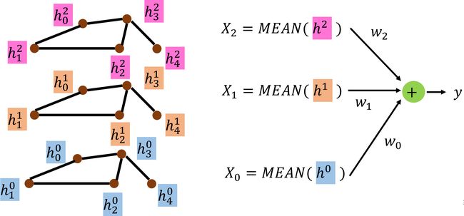
上图说明了 NN4G 做 r e a d o u t readout readout 的过程。求各个 hidden layer 的 hidden feature 的均值 X X X,最后做一个 w e i g h t e d s u m weighted\ sum weighted sum 得到整个图的表示。
DCNN (Diffusion-Convolution Neural Network)
Diffusion-Convolutional Neural Networks (arxiv.org)
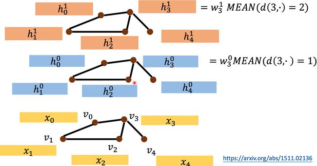
上图说明了 DCNN 在各层计算 hidden feature 的做法。输入依旧是一个 graph,以 h 3 h_3 h3 为例。在 hidden layer 1, h 3 0 = w 3 0 M E A N ( d ( 3 , ⋅ ) = 1 ) h_3^0=w_3^0 MEAN(d(3,\cdot)=1) h30=w30MEAN(d(3,⋅)=1),也就是 h 3 0 h_3^0 h30 由所有距离 node_3 长度为 1 1 1 的结点算均值后再 w e i g h t e d t r a n s f o r m weighted\ transform weighted transform 得到。 h 3 1 h_3^1 h31 也类似可得,只是考虑所有距离 node_3 长度为 2 2 2 的结点。
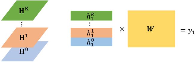
如下图所示,将每层 hidden layer 中的 hidden feature 拼接成一个矩阵 H \bf H H,将这些矩阵 H \bf H H 堆叠起来。如果需要做 Node Classification 的任务,我们只需要取特定的一个 s l i c e slice slice 就能够获得该 node 在各层的 hidden feature,再通过 w e i g h t e d t r a n s f o r m weighted\ transform weighted transform 得到预测的标签。
DGC (Diffusion Graph Convolution)
1707.01926.pdf (arxiv.org) Published as a conference paper in ICLR 2018.
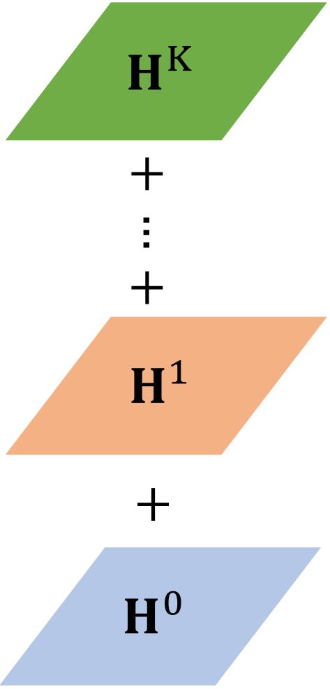
这篇文章没有将矩阵 H \bf H H 堆叠起来,而是将各层的矩阵 H \bf H H 进行相加。
MoNET (Mixture Model Networks)
1611.08402.pdf (arxiv.org)
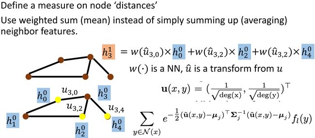
如上图所示,MoNET 设计了一个新的结点间的距离函数: u = ( 1 d e g ( x ) , 1 d e g ( y ) ) T {\bf u}={(\frac{1}{\sqrt {deg(x)}},\ \frac{1}{\sqrt {deg(y)}})}^{\rm T} u=(deg(x)1, deg(y)1)T,度量结点间的距离与两结点的度有关。更新 hidden feature 的方式依旧是对邻居结点做 w e i g h t e d s u m weighted\ sum weighted sum。
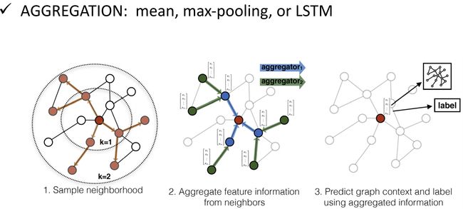
GraphSAGE
1706.02216.pdf (arxiv.org)
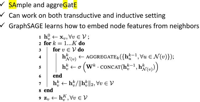
GraphSAGE 做 a g g r e g a t i o n aggregation aggregation 的方式有三种: m e a n , p o o l i n g , L S T M mean,\ pooling,\ LSTM mean, pooling, LSTM。
GAT (Graph Attention Networks)
1710.10903.pdf (arxiv.org) Published as a conference paper at ICLR 2018.
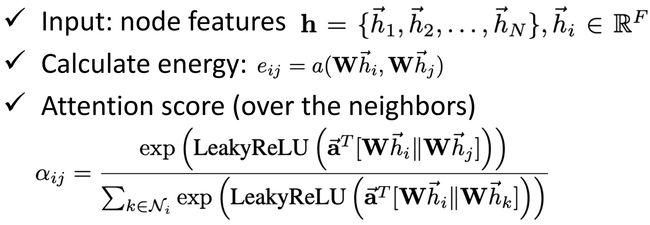

如上图所示,是 GAT 更新 hidden feature 的做法。首先,计算待更新结点 h 3 0 h_3^0 h30 与其邻居结点的 e n e r g y energy energy 值 e 3 , i e_{3,i} e3,i,从而 h 3 1 = e 3 , 0 ⋅ h 0 0 + e 3 , 2 ⋅ h 2 0 + e 3 , 4 ⋅ h 4 0 h_3^1=e_{3,0}\cdot h_0^0+e_{3,2}\cdot h_2^0+e_{3,4}\cdot h_4^0 h31=e3,0⋅h00+e3,2⋅h20+e3,4⋅h40,相当于 a g g r e g a t i o n aggregation aggregation 操作中的 w e i g h t e d s u m weighted\ sum weighted sum 需要学习其中的权重。
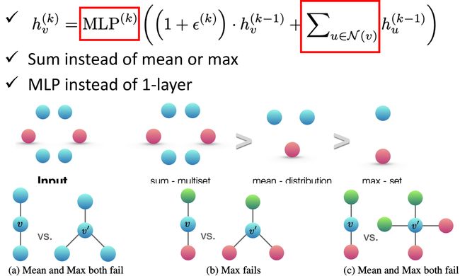
GIN (Graph Isomorphism Network)

Graph Signal Processing and Spectral-based GNN
Spectral-based CNN

对输入、Filter 和 每层的 graph 都做 fourier transform \text{fourier transform} fourier transform 以达到类似于卷积的效果。
Spectral Graph Theory

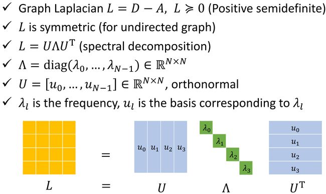
Example

Vertex domain signal
注:由于本人没有学过《信号与系统》,所以以下的内容可能会存在许多错误。(希望有大佬能指出)
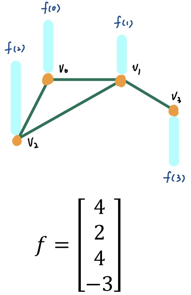
如上图所示,graph 中各个 node 的信号大小由 f f f 给出。那么我们可以得到该 graph 的 adjacency matrix A \bf A A,degree matrix D \bf D D,进而得到 Laplacian L = D − A \bf L=D-A L=D−A(一个半正定 positive semidefinite 矩阵),继续算出 L \bf L L 的特征值(频率 frequency)矩阵 Λ \bf \Lambda Λ 及特征向量组成的矩阵 U \bf U U。
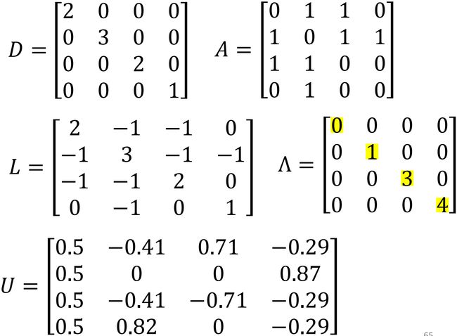
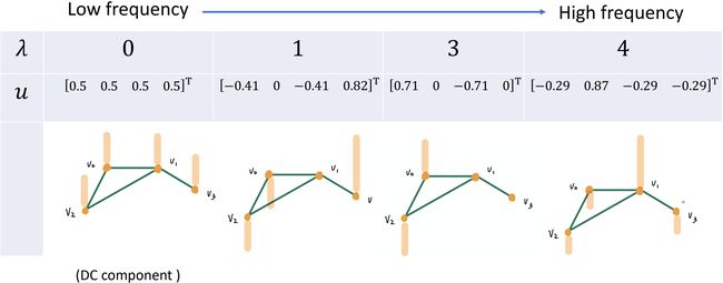
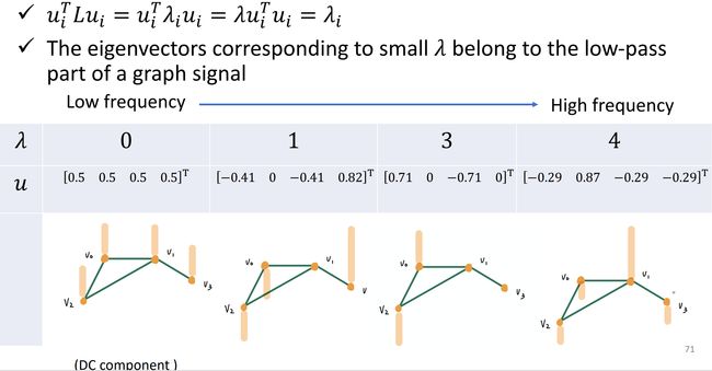
如上图所示,当频率(特征值)分别取 0 , 1 , 3 , 4 0,\ 1,\ 3,\ 4 0, 1, 3, 4 时,各结点的信号强度(用橘黄色标出)。
接下来,我们来尝试理解 vertex frequency:
① 我们可以把 Laplacian L = D − A \bf L=D-A L=D−A 看作作用在图上的一个算子;
② 给定图中的信号 f f f, L f {\bf L}f Lf 代表着什么呢?
③ 简单的数学变换, L f = ( D − A ) f = D f − A f {\bf L}f=({\bf D-A})f={\bf D}f-{\bf A}f Lf=(D−A)f=Df−Af;
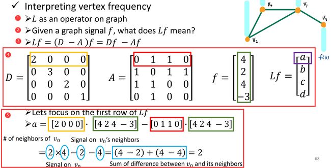
④ 分别写出各结点的 degree matrix D \bf D D,adjacency matrix A \bf A A,假设 f = [ 4 , 2 , 4 , − 3 ] T , L f = [ a , b , c , d ] T f={[4,2,4,-3]}^{\rm T},\ {\bf L}f={[a,b,c,d]}^{\rm T} f=[4,2,4,−3]T, Lf=[a,b,c,d]T;
⑤ 关注 L f {\bf L}f Lf 的第一行,每个蓝圈圈出的数字,其含义如图所示。可以理解成度量某一信号跟他旁边结点的能量差异。
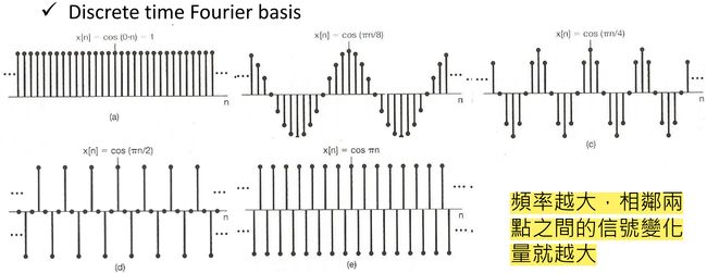
如下图所示,度量信号间能量的差异往往需要将这一差值取平方,进而可以进一步理解为度量图中信号的平滑程度。由 [Spectral Graph Theory](#Spectral Graph Theory),频率越大,相邻两点之间的信号变化量就越大。 f T L f f^{\rm T}{\bf L}f fTLf 代表了不同结点间信号变化量的能量。

用 Laplacian L \bf L L 的特征向量替代 f f f,不难得到下图中的结果。
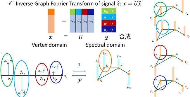
如下图所示,我们想要将 vertex domain 的信号转换到 spectral domain 的信号:
① 类比传统信号与系统中的问题,将方法迁移到我们的问题上来;
② 通过对信号 x x x 的处理: x ^ = U T x \hat x={\bf U}^{\rm T}x x^=UTx,我们可以得到原信号在 spectral domain 的表示,也就是下图中 ③ 这一过程;
④ 那么,如何将 spectral domain 的信号转换到 vertex domain 上呢?依旧类比传统信号与系统中的问题,即下图中 ⑤ 这个过程。
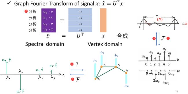
过程 ⑤ 如下图所示:

将过程 ⑤ 拓展到 graph 上,通过对 spectral domain 上的 x ^ \hat x x^ 进行 x = U x ^ x={\bf U}\hat x x=Ux^ 的变换可以完成 spectral domain 到 vertex domain 的信号转换。
Filtering
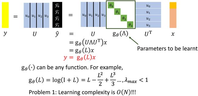
类比传统信号与系统中的问题,对信号进行 Filter —— 乘上一个频率响应的矩阵 g θ {\bf g}_\theta gθ
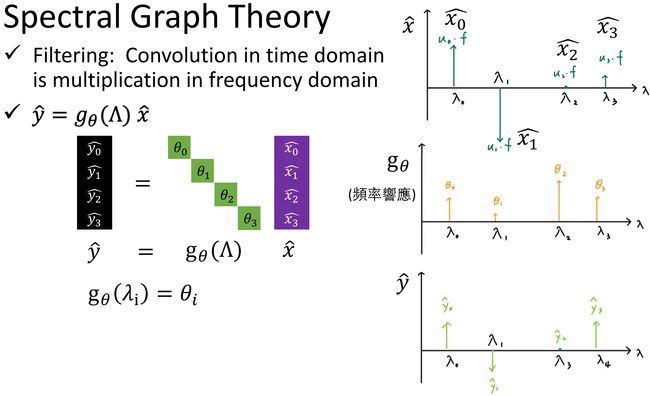
给定输入 x x x,希望模型能够学习到一个 f i l t e r g θ filter\ {\bf g}_\theta filter gθ,输出 y y y,类似于卷积操作。
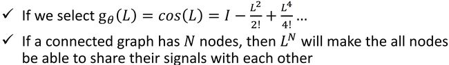
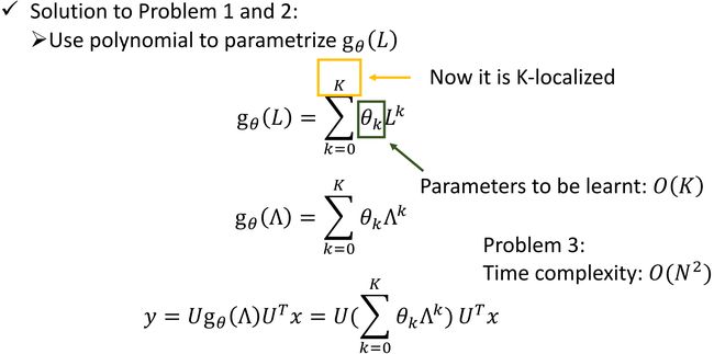
这个模型存在问题,① 学习 g θ {\bf g}_\theta gθ 的复杂度是 O ( N ) O(N) O(N);② 会学习到不应该学习的东西,没有局部化(类比卷积中的 R e c e p t i v e f i e l d Receptive\ field Receptive field,仅对感受野中的数值进行操作,是局部化的操作)。
问题 ② 体现在:
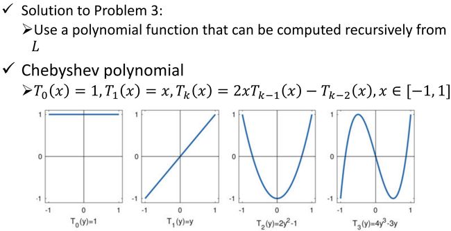
ChebNet
1606.09375.pdf (arxiv.org)
对 g θ {\bf g}_\theta gθ 做出了限制。
GCN