多分类评估指标_评估指标分类

多分类评估指标

If you are familiar with machine learning competitions and you take the time to read through the competition guidelines, you will come across the term Evaluation Metric. The evaluation metric is the basis by which the model performance is determined and winning models placed on the leaderboard. Understanding evaluation metrics will help you build better models and give you an edge over your peers in the event of a competition. We will discuss the common model evaluation metrics paying attention to when they are used, range of values for each metric and most importantly, the values we want to see.

如果您熟悉机器学习竞赛，并且花时间阅读竞赛指南，则会遇到术语“ 评估指标” 。 评估指标是确定模型性能并将获胜模型放置在排行榜上的基础。 了解评估指标将帮助您建立更好的模型，并在竞争中胜过同行。 我们将讨论通用模型评估指标，其中将关注使用它们时，每个指标的值范围以及最重要的是我们希望看到的值。

A prediction model is trained with historical data. To ensure that the model makes accurate predictions — is able to generalize learned rules on new data — the model should be tested using data that it was not trained with.

使用历史数据训练预测模型。 为了确保模型做出准确的预测-能够将学习到的规则推广到新数据上-应该使用未经训练的数据对模型进行测试 。

This can be done by separating the dataset into training data and testing data. The model is trained using the training data and the model’s predictive accuracy is evaluated using the test set. The dataset can be split using sklearn.model_selection.train_test_split from the scikit-learn library.

这可以通过将数据集分为训练数据和测试数据来完成。 使用训练数据对模型进行训练，并使用测试集评估模型的预测准确性。 可以使用sklearn.model_selection拆分数据集。 scikit-learn库中的train_test_split 。

from sklearn.model_selection import train_test_split
X_train, X_test, y_train, y_test = train_test_split(X, y, test_size=0.33)

X is the input feature(s) or independent feature(s)

X是输入要素或独立要素

y is the target column or dependent feature

y是目标列或从属特征

test_size denotes the ratio of total dataset that will be used to test the model.

test_size表示将用于测试模型的总数据集的比率。

The names X_train, X_test, y_train, y_test are conventional names and can be changed to suit your taste.

名称X_train，X_test，y_train，y_test是常规名称，可以更改以适合您的口味。

The model prediction accuracy is then determined using Evaluation Metrics. We will discuss popular evaluation metrics for classification models.

然后，使用评估指标确定模型预测的准确性 。 我们将讨论分类模型的流行评估指标。

混淆矩阵 (Confusion Matrix)

The confusion matrix is a common method that is used to determine and visualize the performance of classification models. The confusion matrix is a NxN matrix where N is the number of target classes or values.

混淆矩阵是用于确定和可视化分类模型性能的常用方法。 混淆矩阵是一个NxN矩阵，其中N是目标类别或值的数量。

The rows in a confusion matrix represent actual values while the columns represent predicted values.

混淆矩阵中的行代表实际值，而列则代表预测值。

混淆矩阵中要注意的术语 (Terms to note in Confusion Matrix)

• True positives: True positives occur when the model has correctly predicted a True instance.

  真实肯定 ：当模型正确预测真实实例时，就会出现真实肯定。

• True Negatives: True negative are cases when the model accurately predicts False instances.

  真否定 ：真否定是模型准确预测False实例的情况。

• False positives: False positives are a situation where the model has predicted a True value when the actual value is False.

  误报 ：误报是当实际值为False时模型已预测为True的情况。

• False negatives: False negative is a situation where the model predicts a False value when the actual value is True.

  假阴性 ：假阴性是当实际值为True时模型预测False值的情况。

To build a better image I will use the Titanic dataset as an example. The Titanic dataset is a popular machine learning dataset and is common amongst beginners. It is a binary classification problem and the goal is to accurately predict which passengers survived the Titanic shipwreck. The passengers who survived are denoted by 1 while the survivors who did not survive are denoted by 0 in the target column SURVIVED.

为了构建更好的图像，我将以Titanic数据集为例。 泰坦尼克号数据集是一种流行的机器学习数据集，在初学者中很常见。 这是一个二元分类问题，目的是准确预测哪些乘客在泰坦尼克号沉船中幸存。 在目标列SURVIVED中，幸存的乘客用1表示，而未幸存的乘客用0表示 。

Now if our model classifies a passenger as having survived (1) and the passenger actually survived (according to our dataset) then that classification is a True Positive — the model accurately predicted a 1.

现在，如果我们的模型将一名乘客分类为已幸存(1)，而该乘客实际上已幸存(根据我们的数据集)，则该分类为“ 真正” —该模型准确地预测为1。

If the model predicts that a passenger did not survive and the passenger did not survive, that is a True Negative classification.

如果模型预测乘客没有幸存且乘客没有幸存，则为真负分类。

But if the model predicts that a passenger survived when the passenger in fact did not survive, that is a case of False Positive.

但是，如果模型预测乘客实际上没有幸存而幸存下来，那就是False Positive的情况。

As you may have guessed, when the model predicts a passenger died when the passenger actually survived, then it is a False Negative.

您可能已经猜到了，当模型预测乘客实际幸存下来而导致乘客死亡时，它就是False Negative 。

Hope this illustration puts things in perspective for you.

希望此插图能为您提供帮助。

An ideal confusion matrix will have higher non-zero values along it’s major diagonal, from left to right.

理想的混淆矩阵沿着其主要对角线(从左到右)将具有更高的非零值。

The Titanic dataset confusion matrix of a Binary Classification problem with only two possible outputs — survived or did not survive — is shown below. We have only two target values, therefore, we have a 2x2 matrix. With the actual values on the vertical axis and the predicted values on the horizontal axis.

下面显示了只有两个可能的输出(幸存或未幸存)的二元分类问题的泰坦尼克数据集混淆矩阵。 我们只有两个目标值，因此，我们有一个2x2矩阵。 纵轴为实际值，横轴为预测值。

Titanic 2x2 Confusion Metric 泰坦尼克号2x2混乱指标

A confusion matrix can also visualize multi-class classification problems. This is not different from the binary classification with the exception of an increase in the dimension of the matrix. A three-class classification problem will have a 3x3 confusion matrix and so on.

混淆矩阵还可以可视化多类分类问题。 这与二进制分类没有什么不同，除了矩阵的维数增加。 三级分类问题将具有3x3混淆矩阵，依此类推。

NxN Confusion Matrix NxN混淆矩阵

Specific Metrics that can be gotten from the Confusion Matrix include:

可以从混淆矩阵中获得的特定指标包括：

准确性 (Accuracy)

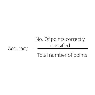
The accuracy metric measures the number of classes that are correctly predicted by the model — the true positives and true negatives.

准确性度量标准衡量模型正确预测的类别的数量-真实肯定和真实否定。

Model Accuracy 模型精度

#calculating accuracy mathematically
Accuracy = sum(clf.predict(X_test)== y_test)/(1.0*len(y_test))#Calculating accuracy using sklearn
from sklearn.metrics import accuracy_score print(accuracy_score(clf.predict(X_test),y_test))

The values for accuracy range from 0 to 1. If a model accuracy is 0, the model is not a good predictor. The accuracy metric is well suited for classification problems where the two classes are balanced or almost balanced.

精度值的范围是0到1 。 如果模型精度为0，则该模型不是良好的预测指标。 精度度量非常适用于两类平衡或几乎平衡的分类问题。

Remember, it is advisable to evaluate the model on new data. If the model is evaluated using the same data the model was trained on, high accuracy value is not surprising as the model remembers the actual values and returns them as predictions. This is called overfitting. Overfitting is a situation whereby the model fits the training data but is not able to accurately predict target values when introduced to new data. To ensure your model is accurate , make sure to evaluate with a new set of data.

请记住，建议根据新数据评估模型。 如果使用与训练模型相同的数据对模型进行评估，则高精度值就不足为奇了，因为模型会记住实际值并将其返回为预测值。 这称为过拟合。 过度拟合是指模型拟合训练数据但当引入新数据时无法准确预测目标值的情况。 为确保模型准确，请确保使用一组新数据进行评估。

精确度和召回率 (Precision and Recall)

The precision and recall metrices work hand-in-hand. While the Precision measures the number of positive values predicted by the model that are actually positive, Recall determines the proportion of the positives values that were accurately predicted.

精度和召回率指标是紧密结合的。 虽然Precision度量模型预测的实际为正的正值的数量，但Recall会确定精确预测的正值的比例。

Precision and Recall 精确度和召回率

A model that produces a low number of false positives has high precision. While a model with low false negatives, has high recall value.

产生少量误报的模型具有较高的精度。 假阴性率低的模型具有较高的召回价值。

Confusion Matrix 混淆矩阵

We will again use the Titanic dataset as before. If the confusion matrix for our model is as above, using our equations above, we get precision and recall values (in 2 dp) as follows:

我们将像以前一样再次使用Titanic数据集。 如果模型的混淆矩阵如上所述，则使用上面的方程式，我们可以得出精度和召回值(以2 dp为单位)，如下所示：

Precision = 0.77

精度= 0.77

Recall = 0.86

召回率= 0.86

If the number of False negatives are decreased, the Recall value increases. Likewise, if the number of False positives is reduced, the precision value increases. From the confusion matrix above, the model is able to predict those who died in the shipwreck more accurately than those who survived.

如果假阴性的数量减少，则调用值会增加。 同样，如果误报的数量减少，则精度值也会增加。 从上面的混淆矩阵中，该模型能够比那些幸存者更准确地预测那些在沉船中丧生的人。

Another way to understand the relationship between precision and recall is with thresholds. The values above the threshold are assigned positive (survived) and values below the threshold are negative (did not survive).

了解精度和召回率之间关系的另一种方法是使用阈值。 高于阈值的值被指定为正(存活)，低于阈值的值被分配为负(未存活)。

If the threshold is 0.5, passengers whose target value fall above 0.5 survived the Titanic. If the threshold is higher, such as 0.8, the accurate number of survivors who survived but are classified as dead will increase (the False Negatives) and the recall value will decrease. At the same time, the number of False positives will reduce as the the model will now classify fewer models as positive due to its high threshold. The Precision value will increase.

如果阈值为0.5，则目标值低于0.5的乘客可以幸免于泰坦尼克号。 如果阈值较高，例如0.8，则存活但被归类为死亡的幸存者的准确数量会增加(假阴性)，召回值会降低。 同时，由于模型的阈值较高，现在该模型将把较少的模型归为阳性，因此误报的数量将减少。 精度值将增加。

In this way, precision and recall can be seen to have a see-saw relationship. If the threshold is lower, the number of positive values increase, the False positive value is higher and the False Negative increases. In his book Hands On Machine Learning with Scikit-Learn, Keras and Tensorflow, Aurélien-Géron describes this Tradeoff splendidly.

这样，可以看到精度和查全率之间存在跷跷板关系。 如果阈值较低，则正值的数量会增加，假正值会更高，而假负数会增加。 Aurélien- Géron在他的《 使用Scikit-Learn，Keras和Tensorflow进行机器学习动手》中出色地描述了这种权衡。

We may choose to focus on precision or recall for a particular problem type. For example, if our model is to classify between malignant cancer and benign cancer, we would want to minimize the chances of a malignant cancer being classified as a benign cancer — we want to minimize the False Negatives — and therefore we can focus on increasing our Recall value rather than Precision. In this situation, we are keen on correctly diagnosing as many malignant cancer as possible, even if some happen to be benign rather than miss a malignant cancer.

对于特定的问题类型，我们可以选择关注精度或召回率。 例如，如果我们的模型是将恶性癌症与良性癌症进行分类，则我们希望将恶性癌症归为良性癌症的机会降到最低–我们希望将假阴性率降到最低，因此我们可以集中精力增加回忆价值而不是精确度。 在这种情况下，即使某些恶性肿瘤是良性的，而不是遗漏了恶性肿瘤，我们仍希望正确诊断出尽可能多的恶性肿瘤。

Precision and Recall values range from 0 to 1 and in both cases, the closer the metric value is to 1, the higher the precision or recall. They are also good metrics to use when the classes are imbalanced and can be averaged for multiclass/multilabel classifications.

精度和查全率值的范围是0到1 ，在两种情况下，度量值越接近1，精度或查全率就越高。 当类不平衡时，它们也是很好的度量标准，可以对多类/多标签分类取平均值。

You can read more on precision and recall in the scikit-learn documentation.

您可以在scikit-learn文档中阅读有关精度和召回的更多信息。

from sklearn.metrics import recall_score
from sklearn.metrics import precision_scorey_test = [0, 1, 1, 0, 1, 0]
y_pred = [0, 0, 1, 0, 0, 1]
recall_score(y_test, y_pred)
precision_score(y_test, y_pred)

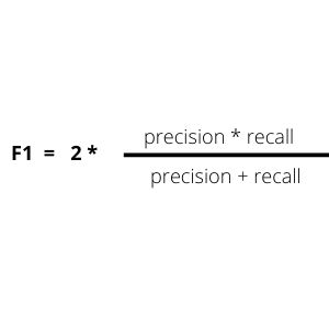
A metric that takes these both precision and recall into consideration is the F1 score.

F1分数是同时考虑到这些准确性和召回率的度量标准。

F1分数 (F1 score)

The F1 score takes into account the precision and recall of the model. The F1 score computes the harmonic mean of precision and recall, giving a higher weight to the low values. Therefore, if either of precision or recall has low values, the F1 score will also have a value closer to the lesser metric. This gives a better model evaluation than an arithmetic mean of precision and recall. A model with high recall and precision values will also have a high F1 score. The F1 score ranges from 0 to 1. The closer the F1 score is to 1, the better the model is.

F1分数考虑了模型的精度和召回率。 F1分数计算精度和查全率的谐波平均值，对较低的值赋予更高的权重。 因此，如果精度或召回率中的任何一个值都较低，则F1得分的值也将更接近较小指标。 与精度和召回率的算术平均值相比，这提供了更好的模型评估。 具有较高召回率和精度值的模型也将具有较高的F1分数。 F1分数的范围是0到1 。 F1分数越接近1，则模型越好。

F1 score also works well with imbalanced classes and for multiclass/multilabel classification targets.

F1分数也适用于不平衡类别以及多类别/多标签分类目标。

from sklearn.metrics import f1_score
f1_score(y_test, y_pred)

F1 score F1分数

To display a summary of the results of the confusion matrix:

要显示混淆矩阵结果的摘要：

from sklearn.metrics import classification_report
y_true = [0, 1, 1, 1, 0]
y_pred = [0, 0, 1, 1, 1]
target_names = ['Zeros', 'Ones']
print(classification_report(y_true, y_pred, target_names=target_names))               precision    recall    f1-score   support       Zeros       0.50      0.50      0.50         2
        Ones       0.67      0.67      0.67         3    accuracy                           0.60         5
   macro avg       0.58      0.58      0.58         5
weighted avg       0.60      0.60      0.60         5

日志损失 (Log Loss)

The Logarithmic Loss metric or Log loss as it’s commonly known, measures how far the predicted values are from the actual values. The Log loss works by penalizing wrong predictions.

对数损耗度量或对数损耗，通常用于衡量预测值与实际值之间的距离。 对数丢失通过惩罚错误的预测而起作用。

Log loss does not have negative values. Its output is a float data type with values ranging from 0 to infinity. A model that accurately predicts the target class has a log loss value close to 0. This indicates that the model has made minimal error in prediction. Log loss is used when the output of the classification model is a probability such as in logistic regression or some neural networks.

对数丢失没有负值。 其输出是float数据类型，其值的范围从0到infinity 。 准确预测目标类别的模型的对数损失值接近0。这表明该模型在预测中的误差很小。 当分类模型的输出是概率时(例如在逻辑回归或某些神经网络中)，将使用对数损失 。

from sklearn.metrics import log_loss
log_loss(y_test, y_pred)

In this post, we have discussed some of the most popular evaluation metrics for a classification model such as the confusion matrix, accuracy, precision, recall, F1 score and log loss. We have seen instances where these metrices are useful and their possible values. We have also outlined the metric scores for each evaluation metric that indicate our model is doing a great job at predicting the actual values. Next time we will look at the charts and curves that can also be used to evaluate the performance of a classification model.

在这篇文章中，我们讨论了分类模型的一些最受欢迎的评估指标，例如混淆矩阵，准确性，精度，召回率，F1得分和对数损失。 我们已经看到了这些指标有用的实例及其可能的值。 我们还概述了每个评估指标的指标得分，这些指标表明我们的模型在预测实际值方面做得很好。 下次，我们将查看可用于评估分类模型性能的图表和曲线。

翻译自: https://medium.com/swlh/evaluation-metrics-i-classification-a26476dd0146

多分类评估指标