2018_WWW_Dual Graph Convolutional Networks for Graph-Based Semi-Supervised Classification

[论文阅读笔记]2018_WWW_Dual Graph Convolutional Networks for Graph-Based Semi-Supervised Classification—(The World Wide Web Conference, 2018.04.23)-- Chenyi Zhuang, Qiang Ma

论文下载地址： https://doi.org/10.1145/3178876.3186116
发表期刊：IW3C2 (International World Wide Web Conference Committee)
Publish time: 2018.04
作者单位: Kyoto University, Kyoto, Japan
数据集：

• 3 个citation network datasets
  • Citeseer
  • Cora
  • Pubmed
• 1个knowledge graph dataset
  • NELL
• Simplified NELL(作者自己根据NELL改的)

代码：

• DGCN: https://github.com/ZhuangCY/Coding-NN
• GCN: https://github.com/tkipf/gcn
• PLANETOID: https://github.com/kimiyoung/planetoid
• DeepWalk: https://github.com/phanein/deepwalk

其他人写的文章

• 《Dual Graph Convolutional Networks for Graph-Based Semi-Supervised Classification》论文理解
• Dual Graph Convolutional Networks for Graph-Based Semi-Supervised Classification
• 点互信息（PMI）和正点互信息（PPMI）

简要概括创新点：(有很多实现的细节，值得去读)

• (1) n this paper, we have proposed a Dual Graph Convolutional Net-work method for graph-based semi-supervised learning. (我们提出了一种基于图的半监督学习的对偶图卷积网络方法)
• (2) In addition to the often-considered local consistency, our method uses the PPMI to encode the global consistency.(除了经常考虑的局部一致性之外，我们的方法还使用PPMI对全局一致性进行编码)
• (3) Our work provides a solution for combining the prior knowledge learned from different views of raw data. (我们的工作为结合从原始数据的不同视图中获得的先验知识提供了一种解决方案。)
• (4) $Con{v}_A$是前人的工作,$Con{v}_P$是本文的创新
• (5) 为了缝合2个部分，提出了一个author设计的Loss函数
• (6) 把NLP中的PPMI拿过来，缝合。为了缝合好，设计了很多细节，包括Random Walk得到频率矩阵$F$,再由$F$得到矩阵$P$.
• (7) adjacency matrix $A$ 和 matrix $P$本质是diffusion
• (8) 自己定义好 context, 和semantic information

Abstract

• (1) we present a simple and scalable semi-supervised learning method(半监督学习) for graph-structured data in which only a very small portion of the training data are labeled.

• (2) In particular, a dual graph convolutional neural network(双图卷积神经网络) method is devised to jointly consider the two essential assumptions of semi-supervised learning:

  • (1) local consistency (这一部分，是前人的工作)
  • (2)and global consistency.(本文创新的着力点)

• (2) Accordingly, two convolutional neural networks are devised to embed the local-consistency-based and global-consistency-based knowledge, respectively。

• (3) Given the different data transformations from the two networks, we then introduce an unsupervised temporal loss function(就是为了缝合2部分神经网络，而设计的) for the ensemble

KeyWords

• Graph convolutional networks,
• Semi-supervised learning,
• Graph diffusion,
• Adjacency matrix,
• Pointwise mutual information

1 Introduction

(第一部分：前人已经做的工作)

• (1) in this paper, we propose a new general semi-supervised learning algorithm that can be applied to different kinds of graphs

• (2) Conventionally, graph-based semi-supervised learning could be defined through the following loss function
  
  where ${\mathcal{L}}_0$ denotes the supervised loss with respect to the labeled data and ${\mathcal{L}}_{reg}$ denotes the regularizer with respect to the graph structure

• (3) ) Using an explicit graph-based regularizer${\mathcal{L}}_{reg}$, the formulation of Eq. (1) smooths the label information in ${\mathcal{L}}_0$ over the whole graph. (式(1)的公式在整个图上平滑了${\mathcal{L}}_0$中的标签信息???)

  • For instance, a graph Laplacian regularization term is typically used in ${\mathcal{L}}_{reg}$ [3] [5] [33], which relies on the prior assumption that connected nodes in the graph are likely to share the same label. (即图中的连通节点可能共享相同的标签)
  • However, this assumption might restrict the modeling capacity, as graph edges need not encode the node similarity, but could instead contain additional information.(种假设可能会限制建模的能力，因为图边不需要编码节点的相似性)

• (4) In Eq. (2), instead of using an explicit graph-based regularizer in the loss function, a convolutional function Conv is derived to encode the graph structure directly.
  

• (5) In approximate terms, the structure encoding Conv could be conducted in two domains:

  • (i) the graph vertex domain [2] [32]; and
  • (ii) the graph spectral domain

the structure encoding Conv

the graph vertex domain

the graph spectral domain

• (6) 前人的不足----->没有考虑global consistency
  However, by using Eqs. (1) and (2), most of the related work have only considered the local consistency of a graph for knowledge embedding. To sufficiently embed the graph knowledge, we find that the global consistency of a graph has not been well investigated yet

(第二部分：在前人的基础上，本文做的工作和创新)

• (7) Hence, in this paper, we propose a dual graph convolutional neural network method to jointly take both of them into consideration.
  The form of the loss function in the proposed strategy is
  
• (8) Using the graph adjacency matrix and positive pointwise mutual information matrix, the two convolutional networks encode the local and global structure information
• (9) Corresponding to the two essential assumptions in semi-supervised learning [32],
  • ConvA embeds the local-consistency-based knowledge (i.e., nearby data points are likely to have the same label),
  • whereas ConvP embeds the global-consistency-based knowledge (i.e., data points that occur in similar contexts tend to have the same label).

2 assumption in semi-supervised learning

ConvA embeds the local-consistency-based knowledge

i.e., nearby data points are likely to have the same label

ConvP embeds the global-consistency-based knowledge

i.e., data points that occur in similar contexts tend to have the same label

• (10) The output of either $Con{v}_A$ or $Con{v}_P$ is then used for supervised learning, e.g., ${\mathcal{L}}_0(Con{v}_A)$.
• (11) However, to give better predictions, an ensemble-oriented regularizer ${\mathcal{L}}_{reg}(Con{v}_A,Con{v}_P)$ for these transformations is derived.
  • By minimizing the difference between predictions from different transformations of an input sample, the regularizer combines the opinions of $Con{v}_A$ and $Con{v}_P$ .
  • Accordingly, ${\mathcal{L}}_{reg}(Con{v}_A,Con{v}_P)$ is an unsupervised loss function

(第三部分：本文Contribution的一个Summary)

• (12) In addition to the graph adjacency matrix-based convolution ConvA,
  • we propose a new convolutional neural network $Con{v}_P$ that depends on the positive pointwise mutual information (PPMI) matrix. (依赖于正点互信息矩阵PPMI)
  • Unlike $Con{v}_A$, which embeds local-consistency-based knowledge,
  • we employ a random walk to construct a PPMI matrix that further embeds semantic information(语义信息), i.e., global-consistency-based knowledge.
• (13) In addition to the supervised learning on a small portion of labeled training data (i.e., $L_0$ in Eq. (3)), (除了对一小部分标注的训练数据(即式(3)中的L0)进行有监督学习外)
  • an unsupervised loss function (i.e., ${\mathcal{L}}_{reg}$ in Eq. (3)) is proposed as a kind of regularizer to combine the output of different convolved data transformations.

2 Background to Graph-based Semi-supervised Learning(是前人的工作，知识基础)

• (1) Semi-supervised learning considers the general problem of learning from labeled and unlabeled data. (半监督学习是干嘛的)
  • Given a set of data points $\mathcal{X}=x_1,...,x_l,x_{l+1},...,x_n$
  • and a set of labels $C=\{1,...,c\}$,
  • the first $l$ points have labels $\{y1,...,yl\}\in C$ and the remaining points are unlabeled.
  • The goal is to predict the labels of the unlabeled points
• (2) In addition to the labeled and unlabeled points, graph-based semisupervised learning
  • also involves a given graph, denoted as an $n\times n$ matrix $A$. Each entry $a_{i,j}\in A$ indicates the similarity between data points $x_i$ and $x_j$
  • the similarity can be derived by calculating the distances among data points [33], or may be explicitly given by structured data, such as knowledge graphs [29], citation graphs [14], hyperlinks between documents [20], and so on
• (3) Therefore, the key problem of graph-based semi-supervised learning concerns how to embed the additional information of the graph for better label prediction.
• (4) In approximate terms, we classify the different graph knowledge embeddings into two groups,
  • i.e., explicit and implicit graph-based semi-supervised learning
  knowledge embeddings

  explicit graph-based semi-supervised learning

  implicit graph-based semi-supervised leraning

2.1 Explicit Graph-based Semi-Supervised Learning

• (1) Explicit graph-based semi-supervised learning uses a graph-based regularizer (i.e., ${\mathcal{L}}_{reg}$ in Eq. (1)) to incorporate the information in the graph.
  

  • Eq. (4) presents an instance of the graph Laplacian regularizer,
  • where $f(\cdot )$ is the label prediction function (e.g., a neural network).
  • The unnormalized graph Laplacian is defined as∆ = A− D,
  • where $A$ is the adjacency matrix and $D$ is a diagonal matrix with each entry defined as $d_{i,j}={\sum }_j{a}_{i,j}$.

• (2) 前人的相似的工作

  • a label propagation algorithm based on Gaussian Random Fields
  • a PageRank-like algorithm is proposed to account for both local and global consistency in the graph
  • a sampling-based method. Instead of using the graph Laplacian∆, they derived a random walk-based sampling algorithm to obtain the positive and negative contexts for each data point
  • a feed-forward neural network method was then used fo knowledge embedding

2.2 Implicit Graph-Based Semi-Supervised Learning

2.2.1 Convolution in the vertex domain(点域的卷积)

• (1) a data point xi will usually be transformed in a diffusive manner. A simple example of a $k$-hop localized linear transform is
  
  where $b_{i,j}$ are some weights for filtering and $\mathcal{N}(i,k)$ denotes the set of neighbors connected to $x_i$ by a path of $k$ or fewer edges.
• (2) Such a convolution is built on the idea of a diffusion kernel, which can be thought of as a measure of the level of connectivity between any two nodes in a grap
  • diffusion-based convolution (基于扩散的卷积)

2.2.2 Convolution in the spectral domain(谱域的卷积)

• (1) We first consider the most simple situation of scalar(标量) $x_i$.
  • In this context, the input $X\in R^{n\times 1}$ is considered as a signal defined on the graph with $n$ nodes
• (2) As shown in Eq. (6), the spectral convolution on a graph can then be defined as the multiplication of the signal $X$ with a filter $g_{\theta }=diag(\theta )$ parametrized by $\theta \in R^n$ in the graph Fourier domain(图傅里叶域)
  
  • where $U$ is the matrix of eigenvectors(特征向量) of the normalized Laplacian matrix(归一化拉普拉斯矩阵)$△=I_n-D^{-\frac{1}{2}}A{D}^{-\frac{1}{2}}$, which plays the role of the Fourier transform
  • when $x_i$ has more than one feature, we can regard $X$ as a signal with multiple input channels.(当有多个特征，就看作是多通道)
  • Eq.(6) is computationally expensive for large graphs.

2.2.3 Realtion between the two domains

• (3) when the filter function $g_{\theta }$ is approximated as an order-$k$ polynomial, the spectral convolution can be interpreted as a k-hop diffusion convolution.
• (4) Thus, by approximating $g_{\theta }$ as an order-1 Chebyshev polynomial(切比雪夫多项式), after some derivation, it is equivalent to a 1-hop diffusion.
• (5) In addition to adjacency matrix-based convolution, we further calculate a PPMI matrix for encoding the semantic information during the convolution.

3 Dual Graph Convolutional Networks(本文设计的模型)

3.1 Problem Definition and an Example

• (1) the input of our model includes
  • a set of data points $\mathcal{X}=\{x_1,...,x_l,x_{l+1},...,x_n\}$
  • the labels {y_1, …, y_l} for the first $l$ points,
  • and the graph structure.
• (2) Assuming that each point has at most $k$ features, the dataset is denoted as a matrix $X\in R^{n\times k}$
• (3) the graph structure is represented by the adjacency matrix $A\in R^{n\times n}$

3.2 Local Consistency Convolution: $Con{v}_A$

3.2这一部分是前人的工作，是一个基础，找到问题，然后提出解决的思路。解决的思路，就是3.3（本文的创新部分）

• (1) we formulate the graph-structure-based convolution $Con{v}_A$ as a type of feed-forward neural network. Given the input feature matrix $X$ and adjacency matrix $A$, the output of the $i$-th hidden layer of the network $Z^{(i)}$ is defined as:
  

  • $\tilde{A}=A+I_n$ , where $I_n\in R^{n\times n}$ is the identity matrix, is the adjacency matrix with self-loops and ${\tilde{D}}_{i,i}={\sum }_j{\tilde{A}}_{i,j}$
  • Accordingly, ${\tilde{D}}^{-\frac{1}{2}}\tilde{A}{\tilde{D}}^{-\frac{1}{2}}$ is the normalized adjacency matrix.
  • $Z^{(i-1)}$ is the output of the $(i-1)$-th layer
  • and $Z^0=X.W^{(i)}$ is the trainable parameters of the network
  • and $\sigma (\cdot )$ denotes an activation function(e.g., ReLU, Sigmoid)

• (2) he role of ${\tilde{D}}^{-\frac{1}{2}}\tilde{A}{\tilde{D}}^{-\frac{1}{2}}{Z}^{(i-1)}$ in Eq. (7) is to exactly conduct a 1-hop diffusion process in each layer. Namely, a node’s feature vector is enriched by linearly adding all the feature vectors of its neighbors. (精确地在每一层进行1跳的扩散过程。即通过将节点相邻节点的所有特征向量线性相加来丰富节点的特征向量)

开始讲故事了

• (3) his discovery inspired the proposed concept. That is, this method can be further improved by reducing the exceptions to local consistency in semi-supervised learning: nearby points are likely to have the same label.(这个发现启发了这个提出的概念。也就是说，该方法可以进一步改进，通过减少半监督学习中局部一致性的异常:附近的点可能有相同的标签.)
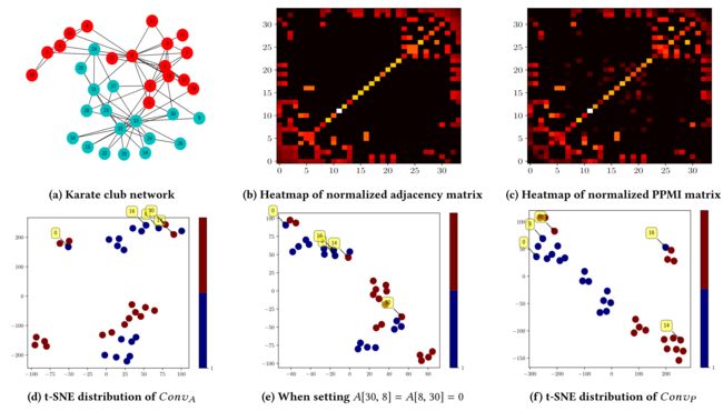
• (4) For example, from Figure 1a, as the directly connected data points $x_8$ and $x_{30}$ have different labels, their convolved feature vectors should not be similar. However, Eq. (7) cannot deal with such an exception in an effective manner.
  (故事的开端，本文为什么要做这件事)
• (5) From the visualized results in Figure 1d, as expected, $x_8$ and $x_{30}$ are close together. However, they belong to different groups. To verify the proposed concept, we manually delete the edge between $x_8$ and $x_{30}$, i.e., setting $A[8,30]=A[30,8]=0$. As a result, Figure 1e presents the new t-SNE distribution of all 34 data points, where $x_8$ and $x_{30}$ are far apart. Hence, the attendant problem is how to automatically reduce the number of such exceptions.(作者猜想，$x_8$ and $x_{30}$之间的边如果删掉，结果就会好。手动删除后，发现真的会好。那作者就要想办法，设计一种Model或者mechanism让程序或者method自动地删除这种情况)
• (6) In the next subsection, we introduce a PPMI-based convolution method.(很自然的引出自己设计的method,开始讲创新点)
  • By encoding semantic information, this method allows different latent representations to be learnt for each data point.(通过对语义信息进行编码，该方法可以为每个数据点学习不同的潜在表示)

3.3 Global Consistency Convolution: $Con{v}_P$

(本文的最大创新点)

• (1) In addition to the graph structure information defined by the adjacency matrix A, we further apply PPMI to encode the semantic information, which is denoted as a matrix $P\in R^{n\times n}$.
• (2) We first calculate a frequency matrix $F$ using a random walk (自己设计的方法)
• (3) Based on F, we then calculate P and explain why it leverages knowledge from the frequency to semantics.(本文的计算流程：先通过Random Walk得到$F$, 再通过$F$去计算$P$)

3.3.1 Calculating frequency matrix $F$(本文创新的模型中，算法流程的起点–Random Walk)

• (1) The Markov chain describing the sequence of nodes visited by a random walker is called a random walk.(描述随机漫步者访问的节点序列的马尔可夫链称为随机漫步。)阐述一下Random Walk是什么

  • If the random walker is on node $x_i$ at time $t$, we define the state as $s(t)=x_i$.
  • The transition probability of jumping from the current node $x_i$ to one of its neighbors $x_j$ is denoted as $p(s(t+1)=x_j|s(t)=x_i)$.

• (2) In our problem setting, given the adjacency matrix $A$, we assign:
  

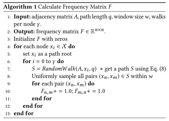
• (3) Algorithm 1 (阐述一些特点)

  • time complexity is $O(n\gamma q^2)$;
  • as the parameters $\gamma$ and $q$ are small integers, $F$ can be calculated quickly.
  • Furthermore, the algorithm could be parallelized by conducting several random walks simultaneously on different parts of a graph(在不同的图上，可以并行)

• (4) Random walks have been used (Random Walk 前人的一些应用)

  • as a similarity measure for a variety of problems in recommendation [11],
  • graph classification [1],
  • and semi-supervised learning [30].
  • In our method, we use a random walk to calculate the semantic similarity between nodes (本文用来计算相似性)

3.3.2 Calculating PPMI

• (1) After calculating the frequency matrix $F$,

  • the $i$-th row in F is the row vector $F_{i,:}$
  • and the $j$-th column in $F$ is the column vector $F_{:,j}$
  • $F_{i,:}$corresponds to a node $x_i$
  • and $F_{:,j}$ corresponds to a context $cj$(本文定义的上下文).

• (2) Based on Algorithm 1,

  • the contexts are defined as all nodes in $\mathcal{X}$.
  • The value of an entry $F_{i,j}$ is the number of times that $x_i$ occurs in context $c_j$

• (3) Based on F, we calculate the PPMI matrix $P\in R^{n\times n}$ as:
  

• (4) Applying Eq. (9) encodes the semantic information in P (通过公式9就得到了语义信息)

  • That is $p_{i,j}$ is the estimated probability that node xi occurs in context $c_j$;
  • $p_{i,\ast }$ is the estimated probability of node $x_i$ ;
  • and $p_{\ast ,j}$ is the estimated probability of context $c_j$
  • Based on the definition of statistical independence, if $x_i$ and $c_j$ are independent (i.e., $x_i)$ occurs in $c_j$ by pure random chance), then $p_{i,j}=p_{i,\ast }{p}_{\ast ,j}$, and thus $pm{i}_{i,j}=0$.
  • Accordingly, if there is a semantic relation between $x_i$ and $c_j$ , then $p_{i,j}$ is expected to be greater than if KaTeX parse error: Expected group after '_' at position 3: xi_̲ and $c_j$ are independent.(相比较于是独立的，有语义联系的话，$p_{i,j}要更大$)
    • Hence, when $p_{i,j}$ > $p_{i,\ast }{p}_{\ast ,j}$ , $pm{i}_{i,j}$ should be positive.(如何区分positive)
    • If node xi is unrelated to context $c_j$ , $pm{i}_{i,j}$ may be negative. (如何区分negative)

• (5) As we are focusing on pairs $(x_i,c_j)$ that have a semantic relation, our method uses a nonnegative $pmi$(本文使用非负的PMI).

• (6) PPMI has been extensively investigated in terms of natural language processing (NLP) (说一下这个想法是从NLP里扒过来的)[4] [16] [28].

  • Indeed, the PPMI metric is known to perform well on semantic similarity tasks

• (7) However, to the best of our knowledge, we are the first to introduce PPMI to the field of graph-based semi-supervised learning.

• (8) Furthermore, using a novel PPMI-based convolution, our method applies the concept of global consistency: graph nodes that occur in similar contexts tend to have the same label.

  • (对比一下PPMI和adjacency的区别)
  • Figure 1c visualizes the normalized PPMI matrix $P$ of the Karate club network.
  • Compared with the adjacency matrix of this network (shown in Figure 1b),
  • there are at least two obvious differences:
    • (1) $P$ has reduced the effect of the hub nodes, e.g., $x_0$ and $x_{33}$; and
    • (2) $P$ has initiated more latent relations among different data points, which cannot be characterized by the adjacency matrix $A$.

3.3.3 PPMI-based convolution

• (1) In addition to the convolution $Con{v}_A$, which is based on the similarity defined by the adjacency matrix $A$, another feed-forward neural network $Con{v}_P$ is derived from the similarity defined by the PPMI matrix $P$.

  本文Model

  Conv_A

  based on the similarity defined by the adjacency matrix A

  Conv_P

  derived from the similarity defined by the PPMI matrix P
  • This convolutional neural network is given by:
    
  • where $P$ is the PPMI matrix and $D_{i,i}={\sum }_j{P}_{i,j}$ for normalization

• (2) Obviously, applying diffusion based on such a node-contextual matrix $P$ ensures global consistency(显然，基于这样的节点上下文矩阵P应用扩散可以确保全局一致性)(自圆其说，支持自己的观点)

• (3) Additionally, by using the same neural network structure as $Con{v}_A$, the two can be combined very concisely. (是一样的神经网络结构，区别是一个基于matrix A, 一个基于matrix P)

• (4) 比较一下 Figure 1f, Figure 1d, Figure1e

3.4 Ensemble of Local and Global Consistencies (得想个办法，把2个部分缝合起来)

• (1) To jointly consider the local consistency and global consistency for semi-supervised learning, we must overcome the challenge of
  • having very few labeled training data(有label的训练数据很少). That is, as the training data are limited, a general ensemble method (e.g., by concatenating the output of ConvA and ConvP ) cannot be utilized. (一般的集成方法不能用)
• (2) supervised learning using training data, we further derive an unsupervised regularizer for the ensemble.(我们进一步推导出一个无监督正则化集成)
  
• (3) Figure 2 presents the architecture of our dual graph convolutional networks method.
  • In addition to training $Con{v}_A$ using the labeled data (i.e., ${\mathcal{L}}_0(Con{v}_A)$ in Eq. (3)
  • an unsupervised regularizer (i.e., ${\mathcal{L}}_{reg}(Con{v}_A,Con{v}_P$ in Eq. (3)) is introduced to train $Con{v}_P$ against the posterior probabilities of a previously trained model, i.e., the trained ${\mathcal{L}}_0(ConvA)$.(无监督正则化被引入，针对之前训练模型的后验概率，去训练$Con{v}_P$)

3.4.1 Calculating ${\mathcal{L}}_0(Con{v}_A)$

• (1) Assuming there are $c$ different labels for prediction(预测$c$个标签),
  • the softmax activation function is applied row-wise to the output $Z^A\in R^{n\times c}$ given by $Con{v}_A$.
  • The output of the softmax layer is denoted as ˆZ A ∈ Rn×c. L0(ConvA), which evaluates the cross-entropy error over all labeled data points, is calculated as:
    
    • where ${\mathcal{Y}}_L$ is the set of data indices whose labels are observed for training
    • and $Y\in R^{n\times c}$ is the ground truth.(真值)

3.4.2 Calculating ${\mathcal{L}}_{reg}(Con{v}_A,Con{v}_P)$

• (1) The calculating of ${\mathcal{L}}_{reg}$ is given by
  

  • Similar to $Con{v}_A$, after applying the softmax activation function, the output of $Con{v}_P$ is denoted as ${\hat{Z}}^P\in R^{n\times c}$
  • Over all $n$ data points, we introduce an unsupervised loss function that minimizes the mean squared differences between ${\hat{Z}}^P$ and ${\hat{Z}}^A$.

• (2) By looking at the formulation of Eq. (12), we could regard the unsupervised loss function as training $Con{v}_P$ against $Con{v}_A$. (我们可以将无监督损失函数视为训练$Con{v}_P$去对抗$Con{v}_A$)

• (3) That is, after the $L_0$-based training (i.e., Eq. (11)), the softmaxed scores in ${\hat{Z}}^A\in R^{n\times c}$ are then interpreted as a posterior distribution over the $c$ labels. (被解释为c个标签之上的后验分布)

  • By minimizing the loss function in .Eq. (12),
  • despite different transformations by $Con{v}_A,Con{v}_P$, and random layer-wise dropout, the final predictions given by each model should then be the same.(每个模型给出的最终预测应该是相同的)

• (4) As shown in Figure 2, the key to our model is to share the model parameters (i.e., neural network weights $W$ in Eqs. (7) and (10)) in $Con{v}_A$ and $Con{v}_P$ .(本文Model的关键就是，2个部分的模型参数共享)

• (5) Although sharing the same parameters $W$ , the different diffusions (i.e., $A$ and $P$)(其实matrix $A$ 和 matrix $P$本质就是一个diffusion) and random dropout may cause the predictions of $Con{v}_A$ and $Con{v}_P$ (i.e., ${\hat{Z}}^A$ and ${\hat{Z}}^P$ ) to differ.

  • However, we know that each data point is assigned to only one class. (每个数据点只分配给一个类)
  • Therefore, the model (which is characterized by the parameters $W$ ) is expected to give the same prediction from $Con{v}_A$ and $Con{v}_P$ , i.e., minimizing Eq. (12). (因此，通过公式(12)，就给出一样的预测了。。。。。)
  • As a result, the trained parameters $W$ have considered the opinions from both $Con{v}_A$ and $Con{v}_P$ .($W$是同时考虑2个部分的得到的)

• (6) By explicitly incorporating the prior knowledge (i.e., the diffusion matrices A and P in our method) during the data transformation stage, (通过在数据转换阶段显式合并先验知识)

  • Namely, by using multiple neural networks, different prior knowledge can be embedded during the data transformation stage.

3.4.3 the final model

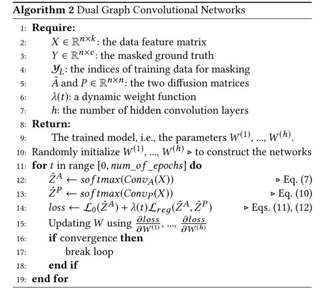
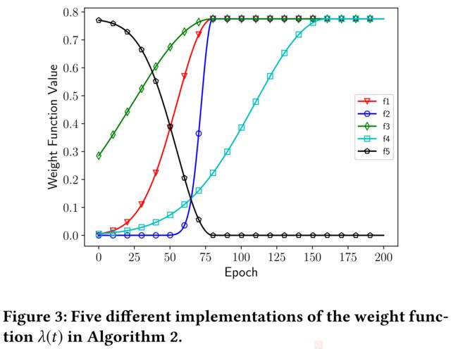
• (1) . Algorithm 2 describes the training process of our dual graph convolutional networks method

  • The loss function is defined as a weighted sum of ${\mathcal{L}}_0(Con{v}_A)$ and ${\mathcal{L}}_{reg}(ConvA,Con{v}_P)$
  • a dynamic weight function is devised to implement the idea described above
    • That is, at the beginning of the training process (i.e., small $t$), the loss function is mainly dominated by the supervised entry $L_0$.
    • After obtaining a posterior distribution over the labels using $Con{v}_A$, increasing $\lambda (t)$ forces our model to simultaneously consider the knowledge encoded in $Con{v}_P$ .(同时考虑$Con{v}_P$)

• (2) our implementation uses Batch Gradient Descent (BGD),

  • in which the full training dataset is used for every training iteration.
  • Although BGD is relatively slow,
  • it is guaranteed to converge to the global minimum for convex error surfaces (但对于凸误差面，它保证收敛到全局最小值)
  • and to a local minimum for non-convex surfaces (对于非凸误差面，它保证收敛到局部最小值)

4 Experiments

4.1 Dataset

• 3 个citation network datasets
  • Citeseer
  • Cora
  • Pubmed
• 1个knowledge graph dataset
  • NELL
• Simplified NELL(作者自己根据NELL改的)

4.1.1 Citeseer

• Only 3.6% of the nodes are labeled for training

4.1.2 Cora

• Only 5.2% of the nodes are labeled for training

4.1.3 Pubmed

• Only 0.3% of the nodes are labeled for training

4.1.4 NELL(Never Ending Language Learning(NELL) knowledge graph)

• each relation in NELL is described as a triplet $(e_h,r,e_t)$
• By spliting each $(e_h,r,e_t)$ into two edges $(e_h,r_1)$ and $(r_2,e_t)$, we obtain a graph …(author自己手动拆分的)
• Only a single data point per class is labeled for training

4.1.5 Simplified NELL

• In simplified NELL, the relation information (i.e., $r$) has been removed and edges among entities have been directly added.
• By counting the co-occurrences of each (eh, et ) pair in all triplets, a weighted adjacency matrix A is constructed.

4.2 Methods for Comparison

4.2.1 DGCN

• (1) This is the proposed method, as described in Algorithm 2. In our Dual Graph Convolutional Networks (DGCN) implementation, both $Con{v}_A$ and $Con{v}_P$ have two hidden layers. (有2层隐藏层)
  • Namely, there are two separate $W$ vectors, $W^{(1)}$ and $W^{(2)}$, that need training in Algorithm 2.
• (2) Table 2 presents detailed information about the implementation of our method for each dataset, including
  • (1) size of the hidden layer;
  • (2) layer-wise dropout rate;
  • (3) window size $w$ in Algorithm 1;and
  • (4) learning rate $\eta$.

4.2.2 GCN(Graph Convolutional Networks)

4.2.3 PLANETOID

• Inspired by the Skipgram model [18] from NLP, PLANETOID [30] embeds the graph information using positive and negative samplings.
  • During sampling, both the label information and graph structure are considered

4.2.4 DeepWalk

• By taking random walks on a graph, different paths are generated.
• By regarding the paths as “sentences, ” DeepWalk [21] generalizes language modeling techniques from sequences of words to paths in a graph. (通过将路径视为“句子”，DeepWalk[21]将语言建模技术从单词序列推广到图中的路径)(因为都是符合某个概率分布的得到的序列)

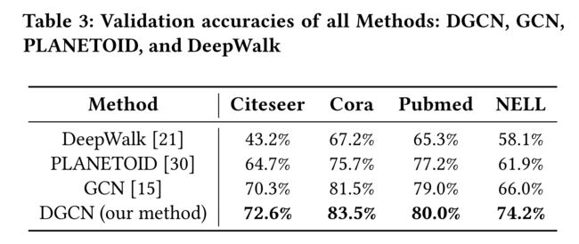
4.3 Results

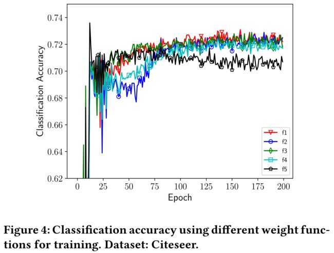
4.4 Effect of Regularization Weight $\lambda (t)$

4.5 4.5 Effect of a Shifted PPMI Matrix $P$

• (1) Eq. (13) presents the calculation of a shifted PPMI matrix, first introduced in [16] for word embedding
• (2) On the basis of the derivation in [16], the value of $k$ indicates the number of negative samplings required to calculate each entry of $P$(k的值表示计算P的每一项所需的负抽样个数)
• (3) In research on semi-supervised learning, we are the first to verify whether such a shift can also be applied to understand a graph.(在半监督学习的研究中，我们首先验证了这种转移是否也可以应用于理解图)

5 Conclusions(大总结，高层次的干货)

• (1) n this paper, we have proposed a Dual Graph Convolutional Net-work method for graph-based semi-supervised learning. (我们提出了一种基于图的半监督学习的对偶图卷积网络方法)
• (2) In addition to the often-considered local consistency, our method uses the PPMI to encode the global consistency.(除了经常考虑的局部一致性之外，我们的方法还使用PPMI对全局一致性进行编码)
• (3) Our work provides a solution for combining the prior knowledge learned from different views of raw data. (我们的工作为结合从原始数据的不同视图中获得的先验知识提供了一种解决方案。)

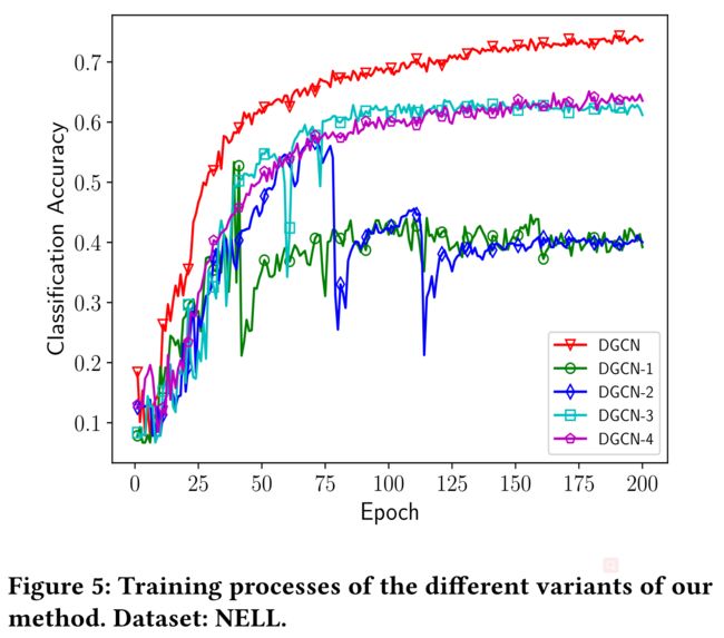
a Variants of our methods(其实就是消融实验)

• DGCN: The original method used in our experiments.
• DGCN-1: When the neural network parameters (i.e., $W^{(h)}s$) are not shared between $Con{v}_A$ and $Con{v}_P$
• DGCN-2: Instead of Eq. (12), we use concatenation to form the ensemble.
  • Namely, the final predictions are derived from the latent representations: $Con{v}_A\oplus Con{v}_P$ . Before softmax, a dense layer is added to ensure the same shape as the label matrix $Y\in R^{n\times c}$
• DGCN-3: When the parameters are not shared between $Con{v}_A$ and $Con{v}_P$ , and concatenation is used.
• DGCN-4: Without ensemble, when only $Con{v}_P$ is used.
  

Acknowledgments

References