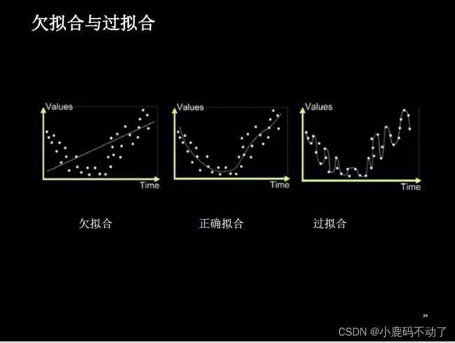
Tensorflow2.0学习教程Class2.5_缓解过拟合
详细学习视频链接:
北京大学


# #p29——free(未添加正则化)(过拟合)
# 导入所需模块
import tensorflow as tf
from matplotlib import pyplot as plt
import numpy as np
import pandas as pd
# 读入数据/标签 生成x_train y_train
df = pd.read_csv('dot.csv')
x_data = np.array(df[['x1', 'x2']])
y_data = np.array(df['y_c'])
x_train = np.vstack(x_data).reshape(-1, 2)
y_train = np.vstack(y_data).reshape(-1, 1)
# print(x_train)
# print(y_train)
Y_c = [['red' if y else 'blue'] for y in y_train]
# 转换x的数据类型,否则后面矩阵相乘时会因数据类型问题报错
x_train = tf.cast(x_train, tf.float32)
y_train = tf.cast(y_train, tf.float32)
# from_tensor_slices函数切分传入的张量的第一个维度,生成相应的数据集,使输入特征和标签值一一对应
train_db = tf.data.Dataset.from_tensor_slices((x_train, y_train)).batch(32)
# 生成神经网络的参数,输入层为2个神经元,隐藏层为11个神经元,1层隐藏层,输出层为1个神经元
# 用tf.Variable()保证参数可训练
w1 = tf.Variable(tf.random.normal([2, 11]), dtype=tf.float32)
b1 = tf.Variable(tf.constant(0.01, shape=[11]))
w2 = tf.Variable(tf.random.normal([11, 1]), dtype=tf.float32)
b2 = tf.Variable(tf.constant(0.01, shape=[1]))
lr = 0.005 # 学习率
epoch = 800 # 循环轮数
# 训练部分
for epoch in range(epoch):
for step, (x_train, y_train) in enumerate(train_db):
with tf.GradientTape() as tape: # 记录梯度信息
h1 = tf.matmul(x_train, w1) + b1 # 记录神经网络乘加运算
h1 = tf.nn.relu(h1)
y = tf.matmul(h1, w2) + b2
# 采用均方误差损失函数mse = mean(sum(y-out)^2)
loss = tf.reduce_mean(tf.square(y_train - y))
# 计算loss对各个参数的梯度
variables = [w1, b1, w2, b2]
grads = tape.gradient(loss, variables)
# 实现梯度更新
# w1 = w1 - lr * w1_grad tape.gradient是自动求导结果与[w1, b1, w2, b2] 索引为0,1,2,3
w1.assign_sub(lr * grads[0])
b1.assign_sub(lr * grads[1])
w2.assign_sub(lr * grads[2])
b2.assign_sub(lr * grads[3])
# 每20个epoch,打印loss信息
if epoch % 20 == 0:
print('epoch:', epoch, 'loss:', float(loss))
# 预测部分
print("*******predict*******")
# xx在-3到3之间以步长为0.01,yy在-3到3之间以步长0.01,生成间隔数值点
xx, yy = np.mgrid[-3:3:.1, -3:3:.1]
# 将xx , yy拉直,并合并配对为二维张量,生成二维坐标点
grid = np.c_[xx.ravel(), yy.ravel()]
grid = tf.cast(grid, tf.float32)
# 将网格坐标点喂入神经网络,进行预测,probs为输出
probs = []
for x_test in grid:
# 使用训练好的参数进行预测
h1 = tf.matmul([x_test], w1) + b1
h1 = tf.nn.relu(h1)
y = tf.matmul(h1, w2) + b2 # y为预测结果
probs.append(y)
# 取第0列给x1,取第1列给x2
x1 = x_data[:, 0]
x2 = x_data[:, 1]
# probs的shape调整成xx的样子
probs = np.array(probs).reshape(xx.shape)
plt.scatter(x1, x2, color=np.squeeze(Y_c)) # squeeze去掉纬度是1的纬度,相当于去掉[['red'],[''blue]],内层括号变为['red','blue']
# 把坐标xx yy和对应的值probs放入contour函数,给probs值为0.5的所有点上色 plt.show()后 显示的是红蓝点的分界线
plt.contour(xx, yy, probs, levels=[.5])
plt.show()
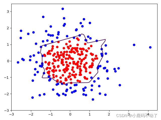
# 读入红蓝点,画出分割线,不包含正则化
# 不清楚的数据,建议print出来查看
产生过拟合现象
# #p29——contain
#读入数据/标签 生成x_data,y_data
df=pd.read_csv('dot.csv')
x_data=np.array(df[['x1','x2']])
y_data=np.array(df['y_c'])
x_train=np.vstack(x_data).reshape(-1,2)
y_train=np.vstack(y_data).reshape(-1,1)
# print(x_train)
# print(y_train)
Y_c = [['red' if y else 'blue'] for y in y_train]
#强制转换数据类型
x_train=tf.cast(x_train,tf.float32)
y_train=tf.cast(y_train,tf.float32)
# from_tensor_slices函数切分传入的张量的第一个维度,生成相应的数据集,使输入特征和标签值一一对应
train_db=tf.data.Dataset.from_tensor_slices((x_train,y_train)).batch(32)
# 生成神经网络的参数,输入层为2个神经元,隐藏层为11个神经元,1层隐藏层,输出层为1个神经元
# 用tf.Variable()保证参数可训练
# 第一层网络
w1=tf.Variable(tf.random.normal([2,11]),dtype=tf.float32)
b1=tf.Variable(tf.constant(0.01,dtype=tf.float32,shape=11))
# print(b1)
# 第二层网络
w2 = tf.Variable(tf.random.normal([11, 1]), dtype=tf.float32)
b2 = tf.Variable(tf.constant(0.01, shape=[1]))
lr=0.005
epoch=1000
#训练部分
for epoch in range(epoch):
for step,(x_train,y_train) in enumerate(train_db):
with tf.GradientTape() as tape: # 记录梯度信息
h1=tf.matmul(x_train,w1)+b1
h1=tf.nn.relu(h1)
y=tf.matmul(h1,w2)+b2
# 发生过拟合:
# # 采用均方误差损失函数mse = mean(sum(y-out)^2)
loss_mse = tf.reduce_mean(tf.square(y_train - y))
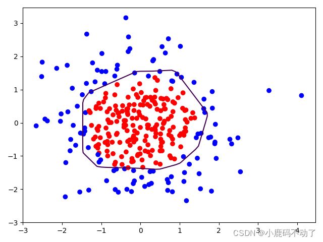
#缓解过拟合:
#添加L2正则化
loss_regularization=[]
# tf.nn.l2_loss(w)=sum(w ** 2) / 2
loss_regularization.append(tf.nn.l2_loss(w1))
loss_regularization.append(tf.nn.l2_loss(w2))
# 求和
# 例:x=tf.constant(([1,1,1],[1,1,1]))
# tf.reduce_sum(x)
# >>>6
# 所有元素求和
loss_regularization=tf.reduce_sum(loss_regularization)
loss=loss_mse+0.03*loss_regularization# REGULARIZER = 0.03
#计算loss对各个参数的梯度
variables=[w1,b1,w2,b2]
grads=tape.gradient(loss,variables)
# 实现梯度更新
# w1 = w1 - lr * w1_grad tape.gradient是自动求导结果与[w1, b1, w2, b2] 索引为0,1,2,3
w1.assign_sub(lr * grads[0])
b1.assign_sub(lr * grads[1])
w2.assign_sub(lr * grads[2])
b2.assign_sub(lr * grads[3])
# 每20个epoch,打印loss信息
if epoch % 20 == 0:
print('epoch:', epoch, 'loss:', float(loss))
# 预测部分
print("*******predict*******")
# xx在-3到3之间以步长为0.01,yy在-3到3之间以步长0.01,生成间隔数值点
xx,yy=np.mgrid[-3:3:.1,-3:3:.1]
#将xx,yy拉直,并合并配对为二维张量,生成二维坐标点
grid=np.c_[xx.ravel(),yy.ravel()]
grid = tf.cast(grid, tf.float32)
# print(grid)
# 将网格坐标点喂入神经网络,进行预测,probs为输出
probs=[]
for x_test in grid:
#使用训练好的参数进行预测
h1=tf.matmul([x_test],w1)+b1
h1=tf.nn.relu(h1)
y=tf.matmul(h1,w2)+b2#预测结果
probs.append(y)
# 取第0列给x1,取第1列给x2
x1 = x_data[:, 0]
x2 = x_data[:, 1]
# probs的shape调整成xx的样子
probs = np.array(probs).reshape(xx.shape)
plt.scatter(x1, x2, color=np.squeeze(Y_c)) # squeeze去掉纬度是1的纬度,相当于去掉[['red'],[''blue]],内层括号变为['red','blue']
# 把坐标xx yy和对应的值probs放入contour函数,给probs值为0.5的所有点上色 plt.show()后 显示的是红蓝点的分界线
plt.contour(xx, yy, probs, levels=[.5])
plt.show()
# 读入红蓝点,画出分割线,不包含正则化
# 不清楚的数据,建议print出来查看
dot.csv
x1,x2,y_c
-0.416757847,-0.056266827,1
-2.136196096,1.640270808,0
-1.793435585,-0.841747366,0
0.502881417,-1.245288087,1
-1.057952219,-0.909007615,1
0.551454045,2.292208013,0
0.041539393,-1.117925445,1
0.539058321,-0.5961597,1
-0.019130497,1.17500122,1
-0.747870949,0.009025251,1
-0.878107893,-0.15643417,1
0.256570452,-0.988779049,1
-0.338821966,-0.236184031,1
-0.637655012,-1.187612286,1
-1.421217227,-0.153495196,0
-0.26905696,2.231366789,0
-2.434767577,0.112726505,0
0.370444537,1.359633863,1
0.501857207,-0.844213704,1
9.76E-06,0.542352572,1
-0.313508197,0.771011738,1
-1.868090655,1.731184666,0
1.467678011,-0.335677339,0
0.61134078,0.047970592,1
-0.829135289,0.087710218,1
1.000365887,-0.381092518,1
-0.375669423,-0.074470763,1
0.43349633,1.27837923,1
-0.634679305,0.508396243,1
0.216116006,-1.858612386,0
-0.419316482,-0.132328898,1
-0.03957024,0.326003433,1
-2.040323049,0.046255523,0
-0.677675577,-1.439439027,0
0.52429643,0.735279576,1
-0.653250268,0.842456282,1
-0.381516482,0.066489009,1
-1.098738947,1.584487056,0
-2.659449456,-0.091452623,0
0.695119605,-2.033466546,0
-0.189469265,-0.077218665,1
0.824703005,1.248212921,0
-0.403892269,-1.384518667,0
1.367235424,1.217885633,0
-0.462005348,0.350888494,1
0.381866234,0.566275441,1
0.204207979,1.406696242,0
-1.737959504,1.040823953,0
0.38047197,-0.217135269,1
1.173531498,-2.343603191,0
1.161521491,0.386078048,1
-1.133133274,0.433092555,1
-0.304086439,2.585294868,0
1.835332723,0.440689872,0
-0.719253841,-0.583414595,1
-0.325049628,-0.560234506,1
-0.902246068,-0.590972275,1
-0.276179492,-0.516883894,1
-0.69858995,-0.928891925,1
2.550438236,-1.473173248,0
-1.021414731,0.432395701,1
-0.32358007,0.423824708,1
0.799179995,1.262613663,0
0.751964849,-0.993760983,1
1.109143281,-1.764917728,0
-0.114421297,-0.498174194,1
-1.060799036,0.591666521,1
-0.183256574,1.019854729,1
-1.482465478,0.846311892,0
0.497940148,0.126504175,1
-1.418810551,-0.251774118,0
-1.546674611,-2.082651936,0
3.279745401,0.97086132,0
1.792592852,-0.429013319,0
0.69619798,0.697416272,1
0.601515814,0.003659491,1
-0.228247558,-2.069612263,0
0.610144086,0.4234969,1
1.117886733,-0.274242089,1
1.741812188,-0.447500876,0
-1.255427218,0.938163671,0
-0.46834626,-1.254720307,1
0.124823646,0.756502143,1
0.241439629,0.497425649,1
4.108692624,0.821120877,0
1.531760316,-1.985845774,0
0.365053516,0.774082033,1
-0.364479092,-0.875979478,1
0.396520159,-0.314617436,1
-0.593755583,1.149500568,1
1.335566168,0.302629336,1
-0.454227855,0.514370717,1
0.829458431,0.630621967,1
-1.45336435,-0.338017777,0
0.359133332,0.622220414,1
0.960781945,0.758370347,1
-1.134318483,-0.707420888,1
-1.221429165,1.804476642,0
0.180409807,0.553164274,1
1.033029066,-0.329002435,1
-1.151002944,-0.426522471,1
-0.148147191,1.501436915,0
0.869598198,-1.087090575,1
0.664221413,0.734884668,1
-1.061365744,-0.108516824,1
-1.850403974,0.330488064,0
-0.31569321,-1.350002103,1
-0.698170998,0.239951198,1
-0.55294944,0.299526813,1
0.552663696,-0.840443012,1
-0.31227067,2.144678089,0
0.121105582,-0.846828752,1
0.060462449,-1.33858888,1
1.132746076,0.370304843,1
1.085806404,0.902179395,1
0.39029645,0.975509412,1
0.191573647,-0.662209012,1
-1.023514985,-0.448174823,1
-2.505458132,1.825994457,0
-1.714067411,-0.076639564,0
-1.31756727,-2.025593592,0
-0.082245375,-0.304666585,1
-0.15972413,0.54894656,1
-0.618375485,0.378794466,1
0.513251444,-0.334844125,1
-0.283519516,0.538424263,1
0.057250947,0.159088487,1
-2.374402684,0.058519935,0
0.376545911,-0.135479764,1
0.335908395,1.904375909,0
0.085364433,0.665334278,1
-0.849995503,-0.852341797,1
-0.479985112,-1.019649099,1
-0.007601138,-0.933830661,1
-0.174996844,-1.437143432,0
-1.652200291,-0.675661789,0
-1.067067124,-0.652931145,1
-0.61209475,-0.351262461,1
1.045477988,1.369016024,0
0.725353259,-0.359474459,1
1.49695179,-1.531111108,0
-2.023363939,0.267972576,0
-0.002206445,-0.139291883,1
0.032565469,-1.640560225,0
-1.156699171,1.234034681,0
1.028184899,-0.721879726,1
1.933156966,-1.070796326,0
-0.571381608,0.292432067,1
-1.194999895,-0.487930544,1
-0.173071165,-0.395346401,1
0.870840765,0.592806797,1
-1.099297309,-0.681530644,1
0.180066685,-0.066931044,1
-0.78774954,0.424753672,1
0.819885117,-0.631118683,1
0.789059649,-1.621673803,0
-1.610499259,0.499939764,0
-0.834515207,-0.996959687,1
-0.263388077,-0.677360492,1
0.327067038,-1.455359445,0
-0.371519124,3.16096597,0
0.109951013,-1.913523218,0
0.599820429,0.549384465,1
1.383781035,0.148349243,1
-0.653541444,1.408833984,0
0.712061227,-1.800716041,0
0.747598942,-0.232897001,1
1.11064528,-0.373338813,1
0.78614607,0.194168696,1
0.586204098,-0.020387292,1
-0.414408598,0.067313412,1
0.631798924,0.417592731,1
1.615176269,0.425606211,0
0.635363758,2.102229267,0
0.066126417,0.535558351,1
-0.603140792,0.041957629,1
1.641914637,0.311697707,0
1.4511699,-1.06492788,0
-1.400845455,0.307525527,0
-1.369638673,2.670337245,0
1.248450298,-1.245726553,0
-0.167168774,-0.57661093,1
0.416021749,-0.057847263,1
0.931887358,1.468332133,0
-0.221320943,-1.173155621,1
0.562669078,-0.164515057,1
1.144855376,-0.152117687,1
0.829789046,0.336065952,1
-0.189044051,-0.449328601,1
0.713524448,2.529734874,0
0.837615794,-0.131682403,1
0.707592866,0.114053878,1
-1.280895178,0.309846277,1
1.548290694,-0.315828043,0
-1.125903781,0.488496666,1
1.830946657,0.940175993,0
1.018717047,2.302378289,0
1.621092978,0.712683273,0
-0.208703629,0.137617991,1
-0.103352168,0.848350567,1
-0.883125561,1.545386826,0
0.145840073,-0.400106056,1
0.815206041,-2.074922365,0
-0.834437391,-0.657718447,1
0.820564332,-0.489157001,1
1.424967034,-0.446857897,0
0.521109431,-0.70819438,1
1.15553059,-0.254530459,1
0.518924924,-0.492994911,1
-1.086548153,-0.230917497,1
1.098010039,-1.01787805,0
-1.529391355,-0.307987737,0
0.780754356,-1.055839639,1
-0.543883381,0.184301739,1
-0.330675843,0.287208202,1
1.189528137,0.021201548,1
-0.06540968,0.766115904,1
-0.061635085,-0.952897152,1
-1.014463064,-1.115263963,0
1.912600678,-0.045263203,0
0.576909718,0.717805695,1
-0.938998998,0.628775807,1
-0.564493432,-2.087807462,0
-0.215050132,-1.075028564,1
-0.337972149,0.343212732,1
2.28253964,-0.495778848,0
-0.163962832,0.371622161,1
0.18652152,-0.158429224,1
-1.082929557,-0.95662552,0
-0.183376735,-1.159806896,1
-0.657768362,-1.251448406,1
1.124482861,-1.497839806,0
1.902017223,-0.580383038,0
-1.054915674,-1.182757204,0
0.779480054,1.026597951,1
-0.848666001,0.331539648,1
-0.149591353,-0.2424406,1
0.151197175,0.765069481,1
-1.916630519,-2.227341292,0
0.206689897,-0.070876356,1
0.684759969,-1.707539051,0
-0.986569665,1.543536339,0
-1.310270529,0.363433972,1
-0.794872445,-0.405286267,1
-1.377757931,1.186048676,0
-1.903821143,-1.198140378,0
-0.910065643,1.176454193,0
0.29921067,0.679267178,1
-0.01766068,0.236040923,1
0.494035871,1.546277646,0
0.246857508,-1.468775799,0
1.147099942,0.095556985,1
-1.107438726,-0.176286141,1
-0.982755667,2.086682727,0
-0.344623671,-2.002079233,0
0.303234433,-0.829874845,1
1.288769407,0.134925462,1
-1.778600641,-0.50079149,0
-1.088161569,-0.757855553,1
-0.6437449,-2.008784527,0
0.196262894,-0.87589637,1
-0.893609209,0.751902355,1
1.896932244,-0.629079151,0
1.812085527,-2.056265741,0
0.562704887,-0.582070757,1
-0.074002975,-0.986496364,1
-0.594722499,-0.314811843,1
-0.346940532,0.411443516,1
2.326390901,-0.634053128,0
-0.154409962,-1.749288804,0
-2.519579296,1.391162427,0
-1.329346443,-0.745596414,0
0.02126085,0.910917515,1
0.315276082,1.866208205,0
-0.182497623,-1.82826634,0
0.138955717,0.119450165,1
-0.8188992,-0.332639265,1
-0.586387955,1.734516344,0
-0.612751558,-1.393442017,0
0.279433757,-1.822231268,0
0.427017458,0.406987749,1
-0.844308241,-0.559820113,1
-0.600520405,1.614873237,0
0.39495322,-1.203813469,1
-1.247472432,-0.07754625,1
-0.013339751,-0.76832325,1
0.29123401,-0.197330948,1
1.07682965,0.437410232,1
-0.093197866,0.135631416,1
-0.882708822,0.884744194,1
0.383204463,-0.416994149,1
0.11779655,-0.536685309,1
2.487184575,-0.451361054,0
0.518836127,0.364448005,1
-0.798348729,0.005657797,1
-0.320934708,0.24951355,1
0.256308392,0.767625083,1
0.783020087,-0.407063047,1
-0.524891667,-0.589808683,1
-0.862531086,-1.742872904,0