【COMP2411: Database Systems Learning Notes】
Database Systems Learning Notes
Resources from the Hong Kong Polytechnic University course COMP2411
Summary
ER model: characterize relationships among entities
Relational model: transform from ER diagram to tables
SQL: language for writing queries
Relational Algebra: logical way to represent queries
Normal Forms: how to design good tables
File Organization: provide file level structure to speed up query (Applications of Index, B+ Tree)
Query Optimization: transform queries into more efficient ones (Calculation, Optimisation graph)
Transactions and Concurrency Control: handle concurrent operations and guarantee correctness of the database
Content
- Summary
- Chapter 1: Database Systems
-
- 1. Introduction
- 2. Database Architecture (1-tier,2-tier,3-tier)
- 3. 3-level Architecture/Three schema Architecture
-
- 1. Internal
- 2. Conceptual
- 3. External
- Mapping
- Data Independence
-
- 1. Logical Data Independence
- 2. Physical Data Independence
- 4. Data Model
- 5. DBMS Language
-
- 5.1 Data Definition Language (DDL)
- 5.2 Data Manipulation Language (DML)
- 6. Data model Schema and Instance
- 7. Basic concepts and terminologies
- Chapter 2: Entity-Relationship (ER) Model
-
- 1. Components of ER diagram
-
- 1. Entity
-
- 1.1.1 Weak Entity
- 2. Attribute
-
- a. Key Attribute
- b. Composite Attribute
- c. Multivalued Attribute
- d. Derived Attribute
- 3. Structural Constraint of relationship: Cardinality ratio (of a binary relationship) V.S. (Min, Max)
-
-
- Relationship V.S. Relationship Sets
- Cardinality ratio
-
- a. One-to-One Relationship (1:1)
- b. One-to-many relationship (1:N)
- c. Many-to-one relationship (N:1)
- d. Many-to-many relationship (M:N)
- Participation constraint (on each participating entity set or type)
-
- Higher degree of relationship
- 2. Notation of ER diagram
- 3. ER Design Issues
-
- 1) Use of Entity Set vs Attributes
- 2) Use of Entity Set vs. Relationship Sets
- 3) Use of Binary vs n-ary Relationship Sets
- 4) Placing Relationship Attributes
- 4. Keys
-
- 1. Primary Keys
- 2. Candidate Keys
- 3. Super Keys
- 4. Foreign Keys
- 5. Generalization
- 6. Specialization
- 7. Aggregation
- 8. Reduction of ER diagram to Table/ ER diagram V.S.
-
- Relational Schema
-
- Method 1
- Method 2
- 9. Relationship of higher degree
- Chapter 3: SQL
-
- Examples
- SELECT `DATA (from bottom to top) SELECT IS THE COLUMN RESULT`
-
- 1. DISTINCT
- 2. AND/OR/NOT
- 3. ORDER BY
- 4. IS NULL/ IS NOT NULL
- 5. TOP
- 6. MIN MAX
- 7. COUNT/AVG/SUM
- 8. LIKE
- 9. IN
- 10. BETWEEN..AND/ NOT BETWEEN..AND
- 11. AS
- 12. ALL and ANY
- AGGREGATE
-
- 13. GROUP BY
- 14. HAVING (with aggregate functions only)
- JOIN
- UNION
- INSERT INTO `DATA (from top to bottom)`
- Lab Java
- 2/11 Discussion
- Chapter 4: Relational Model Concept
-
- 1. Relational Algebra
-
- 1. Select Operation:
- 2. Project Operation
- 3. Union Operation (or):
- 4. Set Intersection (and):
- 5. Set Difference:
- 6. Cartesian product |><|
- 2. Join Operations:
-
- 1. Natural Join
- 2. Outer Join:
-
- a. Left outer join:
- b. Right outer join:
- c. Full outer join:
- 3. Equi join:
- Summary
- Chapter 5: Integrity Constraints (ICs) and Normal Forms
-
- 1. Domain Constraint
- 2. Entity Integrity Constraint
- 3. Referential Integrity Constraint
- 4. Key Constraint
- Functional Dependency and Normal Forms
-
- Types of Functional Dependency
-
- 1. Trivial functional dependency
- 2. Non-trivial functional dependency
- Inference Rules for FDs
-
- 1. Reflexive Rule (IR1)
- 2. Augmentation Rule (IR2)
- 3. Transitive Rule (IR3)
- 4. Union Rule (IR4)
- 5. Decomposition Rule (IR5)
- 6. Pseudo transitive Rule (IR6)
- Types of Normal Forms:
-
- 1NF
-
- Problems
- Solution
- 2NF
- 3NF (Good Design!)
- BCNF
- Chapter 6: File Organization and Indexing
-
- File Organization
- 1. Unordered File
-
- 1.1 Pile File Method:
- 2. Ordered File (Sequential File Organization)
-
- 2.1 Sorted File Method:
- 3. Heap Files (Unordered)
- 4. Hashed Files
-
- 4.1 Static External Hashing
-
- 4.1.1 Collisions problem
-
- 4.1.1.1 Opening Addressing: Linear Probing
- 4.1.1.2 Opening Addressing: Quadratic Probing
- 4.1.2 Overflow chaining/ Overflow handling
- 4.2 Dynamic And Extendible Hashing
- 5. Indexing
-
- 5.1 Ordered indices
-
- 5.1.1 Single level index/ Sparse indexing/ Primary index (Ordered)
-
- 5.1.1.1 Dense index
- 5.1.1.2 Sparse index
- 5.2.1 Clustering index (Ordered)
- 5.3.1 Secondary index (Non-ordered)
- 5.4.1 Multi-level index (primary, secondary, clustering)
- 5.4.2 Using B Trees and B+ Trees as Dynamic Multi-level Indexes
-
- Insertion
- Delection
- Denormalization
- Chapter 7: Query Processing & Query Optimization
-
- 1. Translating SQL Queries into Relational Algebra
- 2. Search Methods for Selection
-
- Linear search (brute force)
- Binary search
- Using a primary index or hash key to retrieve a single record
- Using a primary index to retrieve multiple records
- Using a clustering index to retrieve multiple records
- 3. Calculation
-
- a. Nested-loop join
- b. Block nested-loop join
- c. Merge join
- d. Hash join
- 4. Heuristic Algebraic Optimization Algorithm
- Chapter 8: Transactions and Concurrency Control
-
- 1. Transaction
-
- 1.1 Property of Transaction
- 1.2 Transaction Status
- 2. Schedule
- Example
- 3. Schedules Classified on Recoverability
-
- 3.1 Non-recoverable schedule
- 3.2 Recoverable schedule with cascaded rollback
- 3.3 Cascadeless schedule
- 3.4 Strict schedules
- Example
- 4. Schedules Classified on Serializability
-
- 4.1 Conflict Serializable Schedule
- 4.2 Conflict Equivalent
- 4.3 Result equivalent
- 5. Test of Serializability
-
- 5.1 Non-serializable schedule
- 5.2 Serializable schedule
- Example
- --
- NOT YET MENTIONED IN TGE LECTURE
- View Serializability
- View Equivalent
- --
- Failure Classification
-
- 1. Transaction failure
- 2. System Crash
- 3. Disk Failure
- Log-Based Recovery
-
- Recovery using Log records
- Checkpoint
-
- Recovery using Checkpoint
- Deadlock in DBMS
-
- 1. Deadlock Avoidance
- 2. Deadlock Detection
- 3. Wait for Graph
- Deadlock Prevention
-
- 1. Wait-Die scheme
- 2. Wound wait scheme
- Chapter 8: DBMS Concurrency Control
-
- Concurrent Execution
- Problems with Concurrent Execution
-
- 1. Lost Update Problems (W-W Conflict)
- 2. Dirty Read/ Temporary Update Problems (W-R Conflict)
- 3. Unrepeatable Read Problem (W-R Conflict)
- Concurrency Control Protocols
-
- 1. Lock Based Concurrency Control Protocol
-
- 1. Shared lock
- 2. Exclusive lock
-
- 1. Simplistic lock protocol
- 2. Pre-claiming Lock Protocol
- 3. Two-phase locking (2PL)
- 4. Strict Two-phase locking (Strict-2PL)
- 2. Time Stamp Concurrency Control Protocol
- 3. Validation Based Concurrency Control Protocol
- Multiple Granularity
- Recovery with Concurrent Transaction
- Chapter 9: DDT
- Lab 1 Table Definition, Manipulation and Simple Queries
-
- Link to SQL
- Import .SQL
- Exercise
- 1.1 Common Data Types
- 1.2 NULL values
- 2.1 Inserting Tuples into Tables
- 2.2 Altering Tables
- 3.1 Select
- Lab 2 Queries, Arithmetic Expressions and Functions
-
- 1.1 Selecting Rows within a Certain Range
- 1.2 Selecting Rows That Match a Value in List
- 1.3 Selecting Rows That Match a Character Pattern
- 2.1 Ordering Rows
- 2.2 Ordering Rows Using Multiple Columns
- 2.3 Ordering Rows By Columns With NULL Values
- 3.1 Arithmetic Expressions
- 3.2 Arithmetic Expressions with ORDER BY
- 3.3 The NULL Function
- 3.4 Column Labels
- 4.1 Arithmetic Functions (ROUND)
- 5.1 Character String Functions
- Lab 3 Aggregate Functions, 'Group By' and 'Having' Clauses
-
- 1.1 Selecting Summary Information from One Group
- 2.1 Sub-query
- 2.2 DISTINCT
- 3.1 SELECTING SUMMARY INFORMATION FROM GROUPS – GROUP BY
- 3.2 SPECIFYING A SEARCH-CONDITION FOR GROUPS – HAVING
- 3.3 More on Sub-query
- 4.1 4 EFFECTS OF NULL VALUES ON GROUP FUNCTIONS
- 5 FORMATING QUERY RESULTS INTO A REPORT
Chapter 1: Database Systems
1. Introduction
The main purpose of the database is to operate a large amount of information by storing, retrieving, and managing data.
There are many dynamic websites on the World Wide Web nowadays which are handled through databases. For example, a model that checks the availability of rooms in a hotel. It is an example of a dynamic website that uses a database.
There are many databases available like MySQL, Sybase, Oracle, MongoDB, Informix, PostgreSQL, SQL Server, etc.
Relational Database
Relational database model has two main terminologies called instance and schema.
The instance is a table with rows or columns
There are following four commonly known properties of a relational model known as ACID properties, where:
A means Atomicity: This ensures the data operation will complete either with success or with failure. It follows the ‘all or nothing’ strategy. For example, a transaction will either be committed or will abort.
C means Consistency: If we perform any operation over the data, its value before and after the operation should be preserved. For example, the account balance before and after the transaction should be correct, i.e., it should remain conserved.
I means Isolation: There can be concurrent users for accessing data at the same time from the database. Thus, isolation between the data should remain isolated. For example, when multiple transactions occur at the same time, one transaction effects should not be visible to the other transactions in the database.
D means Durability: It ensures that once it completes the operation and commits the data, data changes should remain permanent.
Cloud Database
Cloud database facilitates you to store, manage, and retrieve their structured, unstructured data via a cloud platform. This data is accessible over the Internet. Cloud databases are also called a database as service (DBaaS) because they are offered as a managed service.
e.g., DWS, Oracle, MS Server
NoSQL
Not only for database
MongoDB, CouchDB, Cloudant (Document-based)
Memcached, Redis, Coherence (key-value store)
HBase, Big Table, Accumulo (Tabular)
DBMS, Graph Database, RDBMS…
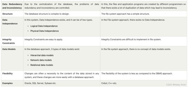
DBMS VS RDBMS

DBMS VS File System
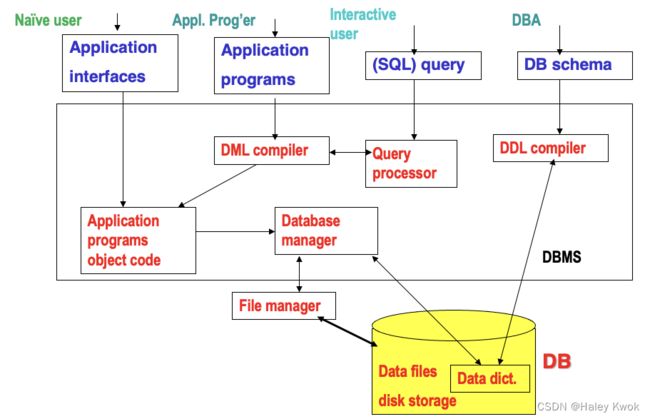
2. Database Architecture (1-tier,2-tier,3-tier)
2-tier Architecture
The 2-Tier architecture is same as basic client-server. In the two-tier architecture, applications on the client end can directly communicate with the database at the server side. For this interaction, API’s like: ODBC, JDBC are used.
The user interfaces and application programs are run on the client-side.
The server side is responsible to provide the functionalities like: query processing and transaction management.
To communicate with the DBMS, client-side application establishes a connection with the server side.

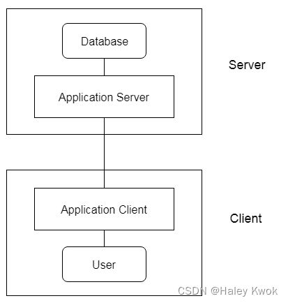
3-tier Architecture
The 3-Tier architecture contains another layer between the client and server. In this architecture, client can’t directly communicate with the server.
The application on the client-end interacts with an application server which further communicates with the database system.
End user has no idea about the existence of the database beyond the application server. The database also has no idea about any other user beyond the application.
The 3-Tier architecture is used in case of large web application.
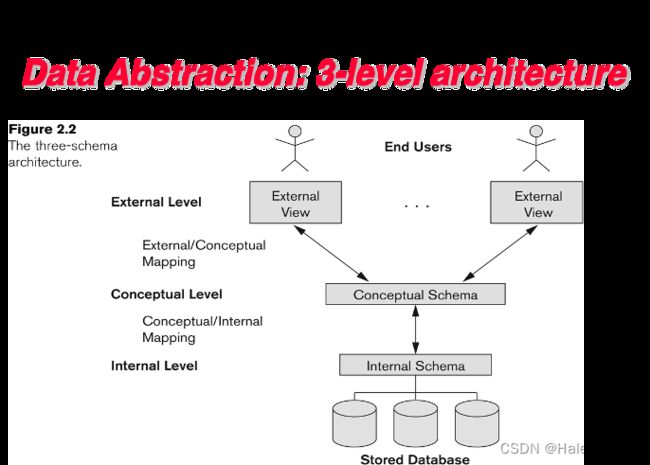
3. 3-level Architecture/Three schema Architecture
The three schema architecture is also called ANSI/SPARC architecture or three-level architecture.
The main objective of three level architecture is to enable multiple users to access the same data with a personalized view while storing the underlying data only once. Thus it separates the user’s view from the physical structure of the database.
- Abstract view of the data
simplify interaction with the system
hide details of how data is stored and manipulated - Levels of abstraction
physical/internal level: data structures; how data are actually stored
conceptual level: schema, what data are actually stored
view/external level: partial schema - the ability to manage persistent data
- primary goal of DBMS: to provide an environment that is convenient, efficient, and robust to use in retrieving & storing data
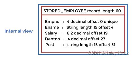
1. Internal
How data store in block
Storage space allocations.
For Example: B-Trees, Hashing etc.
Access paths.
For Example: Specification of primary and secondary keys, indexes, pointers and sequencing.
Data compression and encryption techniques.
Optimization of internal structures.
Representation of stored fields.
2. Conceptual
The conceptual schema describes the design of a database at the conceptual level. Conceptual level is also known as logical level.
The conceptual schema describes the structure of the whole database.
The conceptual level describes what data are to be stored in the database and also describes what relationship exists among those data.
In the conceptual level, internal details such as an implementation of the data structure are hidden.
Programmers and database administrators work at this level.

3. External
At the external level, a database contains several schemas that sometimes called as subschema. The subschema is used to describe the different view of the database.
An external schema is also known as view schema.
Each view schema describes the database part that a particular user group is interested and hides the remaining database from that user group.
The view schema describes the end user interaction with database systems.
![]()
Mapping
- Conceptual/ Internal Mapping
The Conceptual/ Internal Mapping lies between the conceptual level and the internal level. Its role is to define the correspondence between the records and fields of the conceptual level and files and data structures of the internal level.
- External/ Conceptual Mapping
The External/Conceptual Mapping lies between the external level and the Conceptual level. Its role is to define the correspondence between a particular external and the conceptual view.
Data Independence
Data independence can be explained using the three-schema architecture.
Data independence refers characteristic of being able to modify the schema at one level of the database system without altering the schema at the next higher level.
There are two types of data independence:
1. Logical Data Independence
Logical data independence refers characteristic of being able to change the conceptual schema without having to change the external schema.
Logical data independence is used to separate the external level from the conceptual view.
If we do any changes in the conceptual view of the data, then the user view of the data would not be affected.
Logical data independence occurs at the user interface level.
2. Physical Data Independence
Physical data independence can be defined as the capacity to change the internal schema without having to change the conceptual schema.
If we do any changes in the storage size of the database system server, then the Conceptual structure of the database will not be affected.
Physical data independence is used to separate conceptual levels from the internal levels.
Physical data independence occurs at the logical interface level.
4. Data Model
- Object-based logical models (conceptual & view levels)
the Entity-Relationship (ER) model – mid 70’s
the Semantic Data Models – early/mid 80’s
the Object-Oriented data models – late 80’s - Record-based logical models (conceptual & view levels)
the Network and Hierarchical models – 60’s
the Relational model – early 70’s
An ER model is the logical representation of data as objects and relationships among them. These objects are known as entities, and relationship is an association among these entities. This model was designed by Peter Chen and published in 1976 papers. It was widely used in database designing. A set of attributes describe the entities. For example, student_name, student_id describes the ‘student’ entity. A set of the same type of entities is known as an 'Entity set', and the set of the same type of relationships is known as 'relationship set'.
5. DBMS Language

5.1 Data Definition Language (DDL)
- a language for defining DB schema
- Data definition language is used to
store the information of metadatalike the number of tables and schemas, their names, indexes, columns in each table, constraints, etc.
Create: It is used to create objects in the database.
Alter: It is used to alter the structure of the database.
Drop: It is used to delete objects from the database.
Truncate: It is used to remove all records from a table.
Rename: It is used to rename an object.
Comment: It is used to comment on the data dictionary.
These commands are used to update the database schema that’s why they come under Data definition language.
5.2 Data Manipulation Language (DML)
DML stands for Data Manipulation Language. It is used for accessing and manipulating data in a database. It handles user requests.
- an important subset for retrieving data is called Query Language
- two types of DML: procedural (specify “what” & “how”) vs. declarative (just specify “what”)
Select: It is used to retrieve data from a database.
Insert: It is used to insert data into a table.
Update: It is used to update existing data within a table.
Delete: It is used to delete all records from a table.
Merge: It performs UPSERT operation, i.e., insert or update operations.
Call: It is used to call a structured query language or a Java subprogram.
Explain Plan: It has the parameter of explaining data.
Lock Table: It controls concurrency.
6. Data model Schema and Instance
The data which is stored in the database at a particular moment of time is called an instance of the database.
The overall design of a database is called schema.
A database schema is the skeleton structure of the database. It represents the logical view of the entire database.
A schema contains schema objects like table, foreign key, primary key, views, columns, data types, stored procedure, etc.
A database schema can be represented by using the visual diagram. That diagram shows the database objects and relationship with each other.
7. Basic concepts and terminologies
- instance
the collection of data (information) stored in the DB at a particular moment (ie, a snapshot) - scheme/schema
the overall structure (design) of the DB – relatively static
Chapter 2: Entity-Relationship (ER) Model
1. Components of ER diagram

1. Entity
An entity may be any object, class, person or place. In the ER diagram, an entity can be represented as rectangles.
Consider an organization as an example- manager, product, employee, department etc. can be taken as an entity.

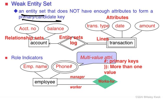
1.1.1 Weak Entity
An entity that depends on another entity called a weak entity. The weak entity doesn’t contain any key attribute of its own. The weak entity is represented by a double rectangle.

There is no primary key in weak attribute (non-key attribute)


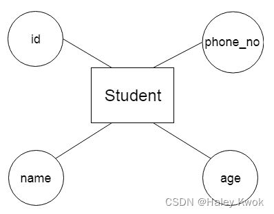
2. Attribute
The attribute is used to describe the property of an entity. Eclipse is used to represent an attribute.
For example, id, age, contact number, name, etc. can be attributes of a student.
a. Key Attribute
The key attribute is used to represent the main characteristics of an entity. It represents a primary key. The key attribute is represented by an ellipse with the text underlined.
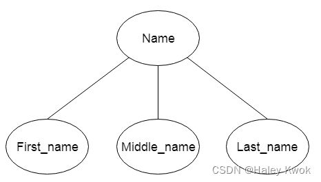
b. Composite Attribute
An attribute that composed of many other attributes is known as a composite attribute. The composite attribute is represented by an ellipse, and those ellipses are connected with an ellipse.
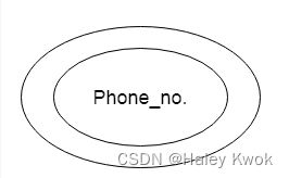
c. Multivalued Attribute
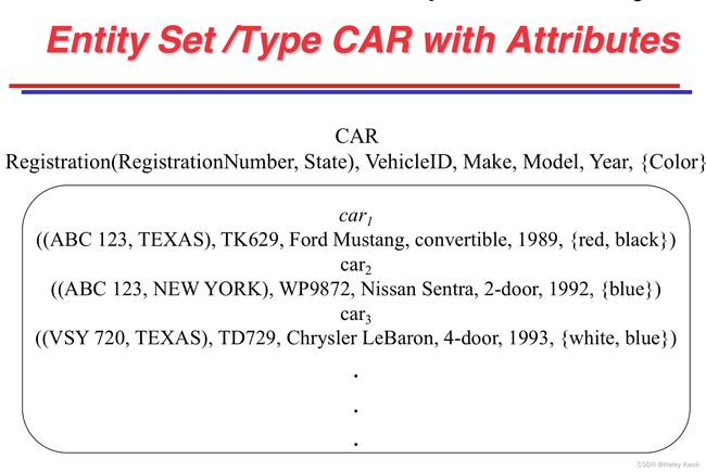
An attribute can have more than one value. These attributes are known as a multivalued attribute. The double oval is used to represent multivalued attribute. For example, a student can have more than one phone number.
SIMPLE: SSN, Sex
COMPOSITE: Address(Apt#, Street, City, State, ZipCode, Country) or Name(FirstName, MiddleName, LastName)
MULTI-VALUED: multiple values; Color of a CAR, denoted as {Color}.
COMPOSITE and MULTI-VALUED may be generally nested.
{PreviousDegrees(College, Year, Degrees, Field)}
d. Derived Attribute
An attribute that can be derived from other attribute is known as a derived attribute. It can be represented by a dashed ellipse. For example, A person’s age changes over time and can be derived from another attribute like Date of birth.

3. Structural Constraint of relationship: Cardinality ratio (of a binary relationship) V.S. (Min, Max)
Relationship V.S. Relationship Sets
- Relationship: related two or more distinct entities with a specific meaning
EMPLOYEE John Smithworks onthe PROJECT ‘solar’, or EMPLOYEE Franklin Wongmanagesthe Research DEPARTMENT. - Relationship Set: Relationships of the same type are grouped together.
theWORKS_ONrelationship type in which EMPLOYEES and PROJECTS participate; theMANAGESrelationship type in which EMPLOYEE and DEPARTMENT.
Both MANAGES and WORKS_ON are binary relationships, both of which can same participate in entity sets/ types.
Cardinality ratio
A relationship is used to describe the relation between entities. Diamond or rhombus is used to represent the relationship.
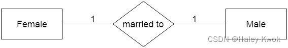
a. One-to-One Relationship (1:1)
When only one instance of an entity is associated with the relationship, then it is known as one to one relationship.
For example, A female can marry to one male, and a male can marry to one female.
b. One-to-many relationship (1:N)
When only one instance of the entity on the left, and more than one instance of an entity on the right associates with the relationship then this is known as a one-to-many relationship.
For example, Scientist can invent many inventions, but the invention is done by the only specific scientist.

c. Many-to-one relationship (N:1)
When more than one instance of the entity on the left, and only one instance of an entity on the right associates with the relationship then it is known as a many-to-one relationship.
For example, Student enrolls for only one course, but a course can have many students.

d. Many-to-many relationship (M:N)
When more than one instance of the entity on the left, and more than one instance of an entity on the right associates with the relationship then it is known as a many-to-many relationship.
For example, Employee can assign by many projects and project can have many employees.

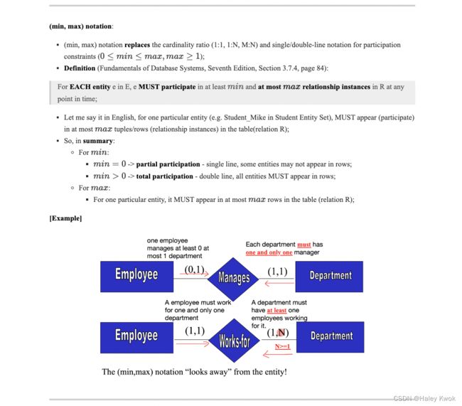
Participation constraint (on each participating entity set or type)
Partial participation: min = 0, MAY NOT appears in the rows; by single line
Total participation: min > 0, MUST appears in the rows; by double line (every entity participate)
Minimum cardinality tells whether the participation is partial or total.
If minimum cardinality = 0, then it signifies partial participation.
If minimum cardinality = 1, then it signifies total participation.
Maximum cardinality tells the maximum number of entities that participates in a relationship set.
Higher degree of relationship
Directly transformation between cardinality ratio and ( m i n , m a x ) (min, max) (min,max) is not allowed.
(MIN, MAX) can be considered as how many times an entity would appear in the rows.

[Examples]
One-to-one
Many students belong to one department
Student ---- N ----- belongs to ----- 1 ---- Department
Each student belongs to at one department only; Each department has at least one and more than one students
This would be more clear, since some times when there is tertinary relationship, m:n:p is meaningless.
Student ---- ( 1,1 ) ----- belongs to -----( 1,N ) ---- Department
2. Notation of ER diagram

3. ER Design Issues
1) Use of Entity Set vs Attributes
The use of an entity set or attribute depends on the structure of the real-world enterprise that is being modelled and the semantics associated with its attributes. It leads to a mistake when the user use the primary key of an entity set as an attribute of another entity set. Instead, he should use the relationship to do so. Also, the primary key attributes are implicit in the relationship set, but we designate it in the relationship sets.
We should not link ____ directly with other entity’s attribute
2) Use of Entity Set vs. Relationship Sets
It is difficult to examine if an object can be best expressed by an entity set or relationship set. To understand and determine the right use, the user need to designate a relationship set for describing an action that occurs in-between the entities.
If there is a requirement of representing the object as a relationship set, then its better not to mix it with the entity set.
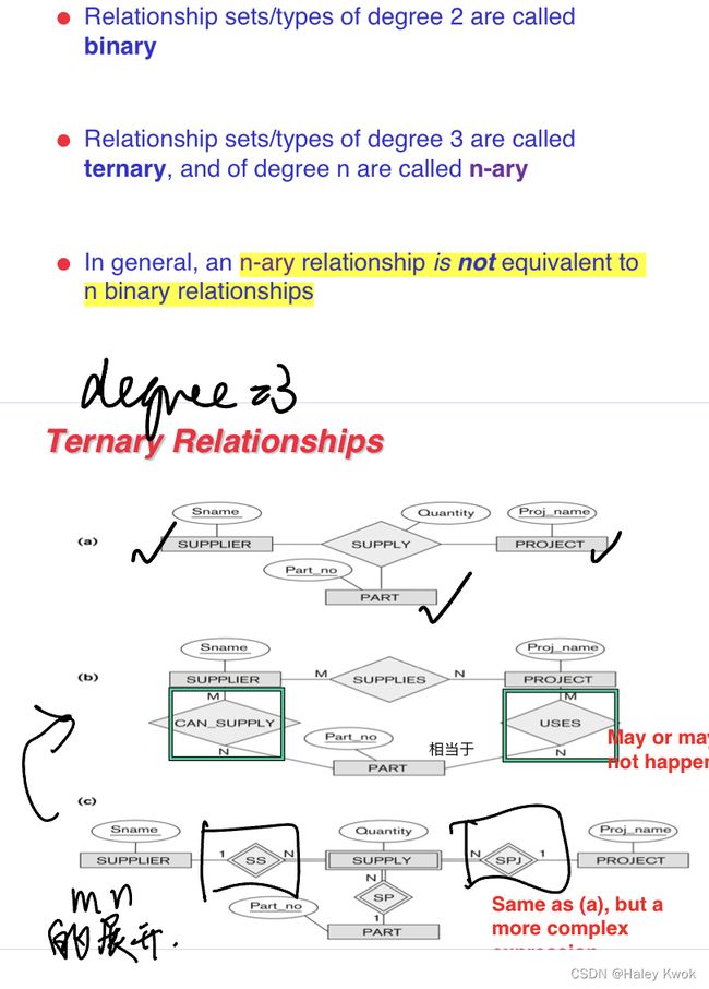
3) Use of Binary vs n-ary Relationship Sets
Generally, the relationships described in the databases are binary relationships. However, non-binary relationships can be represented by several binary relationships. For example, we can create and represent a ternary relationship ‘parent’ that may relate to a child, his father, as well as his mother. Such relationship can also be represented by two binary relationships i.e, mother and father, that may relate to their child.
It is possible to represent a non-binary relationship by a set of distinct binary relationships.


4) Placing Relationship Attributes
The cardinality ratios can become an affective measure in the placement of the relationship attributes. So, it is better to associate the attributes of one-to-one or one-to-many relationship sets with any participating entity sets, instead of any relationship set. The decision of placing the specified attribute as a relationship or entity attribute should possess the charactestics of the real world enterprise that is being modelled.
For example, if there is an entity which can be determined by the combination of participating entity sets, instead of determing it as a separate entity. Such type of attribute must be associated with the many-to-many relationship sets.
Focus on the number of determination
4. Keys
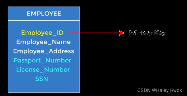
1. Primary Keys
The minimal attribute of candidate key, which is the first key used to identify one and only one instance of an entity uniquely. An entity can contain multiple keys, as we saw in the PERSON table. The key which is most suitable from those lists becomes a primary key.
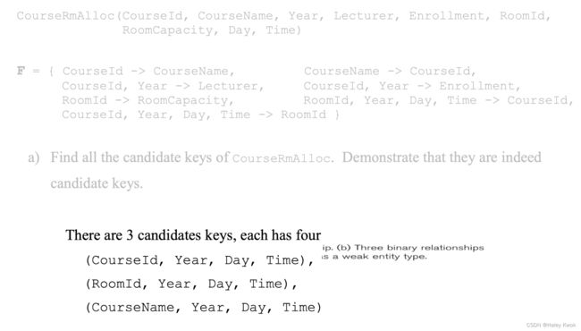
2. Candidate Keys
A candidate key is an attribute or set of attributes that can uniquely identify a tuple.
Except for the primary key, the remaining attributes are considered a candidate key. The candidate keys are as strong as the primary key.
For example: In the EMPLOYEE table, id is best suited for the primary key. The rest of the attributes, like SSN, Passport_Number, License_Number, etc., are considered a candidate key.

3. Super Keys
Super key is an attribute set that can uniquely identify a tuple. A super key is a superset of a candidate key.
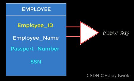
For example: In the above EMPLOYEE table, for(EMPLOEE_ID, EMPLOYEE_NAME), the name of two employees can be the same, but their EMPLYEE_ID can’t be the same. Hence, this combination can also be a key.
The super key would be EMPLOYEE-ID (EMPLOYEE_ID, EMPLOYEE-NAME), etc.
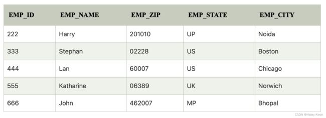
Super key in the table above:
{EMP_ID}, {EMP_ID, EMP_NAME}, {EMP_ID, EMP_NAME, EMP_ZIP}…so on
Candidate key: {EMP_ID}
To find the candidate keys, you need to see what path leads you to all attributes using the dependencies. So you are correct about A because from A you can reach B that can reach {C, D}. AB can’t be considered a candidate key because it has never been mentioned in your dependencies. Another way to think about it is by remembering that candidate key is the minimum number of attributes that guarantees uniqueness in your rows. But since A is already a candidate key then AB is not minimal set. Since you only have one candidate key that’s A. A is called a key attribute and all other attributes are called non-key attributes. then you decide the number of super keys by 2 to the power of number of non-key attributes (B, C, D). In this scenario you should have 8 super keys. The way to find them is simply by mashing A with all possible combinations of the non-key attributes. So your superkeys would be A, AB, AC, AD, ABC, ABD, ACD, ABCD.
Find the Superkeys
4. Foreign Keys
Foreign keys are the column of the table used to point to the primary key of another table.
Every employee works in a specific department in a company, and employee and department are two different entities. So we can’t store the department’s information in the employee table. That’s why we link these two tables through the primary key of one table.
We add the primary key of the DEPARTMENT table, Department_Id, as a new attribute in the EMPLOYEE table.
In the EMPLOYEE table, Department_Id is the foreign key, and both the tables are related.

3 more keys to go…
superkey
a set of one or more attributes which, taken together, identify uniquely an entity in an entity set
Example: {student ID, Name} identify a student
candidate key
minimal set of attributes which can identify uniquely an entity in an entity set
a special case of superkey (for which no proper subset is a superkey)
Example: student ID identify a student, but Name is not a candidate key (WHY?)
more than candidate key, pick one as primary key
primary key
a candidate key chosen by the DB designer to identify an entity in an entity set
5. Generalization
Generalization is like a bottom-up approach in which two or more entities of lower level combine to form a higher level entity if they have some attributes in common.
In generalization, an entity of a higher level can also combine with the entities of the lower level to form a further higher level entity.
Generalization is more like subclass and superclass system, but the only difference is the approach. Generalization uses the bottom-up approach.
In generalization, entities are combined to form a more generalized entity, i.e., subclasses are combined to make a superclass.
For example, Faculty and Student entities can be generalized and create a higher level entity Person.

6. Specialization
Specialization is a top-down approach, and it is opposite to Generalization. In specialization, one higher level entity can be broken down into two lower level entities.
Specialization is used to identify the subset of an entity set that shares some distinguishing characteristics.
Normally, the superclass is defined first, the subclass and its related attributes are defined next, and relationship set are then added.
For example: In an Employee management system, EMPLOYEE entity can be specialized as TESTER or DEVELOPER based on what role they play in the company.

7. Aggregation
In aggregation, the relation between two entities is treated as a single entity. In aggregation, relationship with its corresponding entities is aggregated into a higher level entity.
For example: Center entity offers the Course entity act as a single entity in the relationship which is in a relationship with another entity visitor. In the real world, if a visitor visits a coaching center then he will never enquiry about the Course only or just about the Center instead he will ask the enquiry about both.

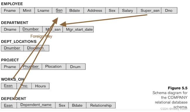
8. Reduction of ER diagram to Table/ ER diagram V.S.
The database can be represented using the notations, and these notations can be reduced to a collection of tables.
In the database, every entity set or relationship set can be represented in tabular form.

In the student table, a hobby is a multivalued attribute. So it is not possible to represent multiple values in a single column of STUDENT table.

Don't have to link the arrow, since it is not the referential constraints
Entity: EMPLOYEE, DEPARTMENT, PROJECT, DEPENDENT
Relationship: DEPT_LOCATIONS, WORKS_ON -> primary keys, and non-key attributes
Relational Schema
Method 1
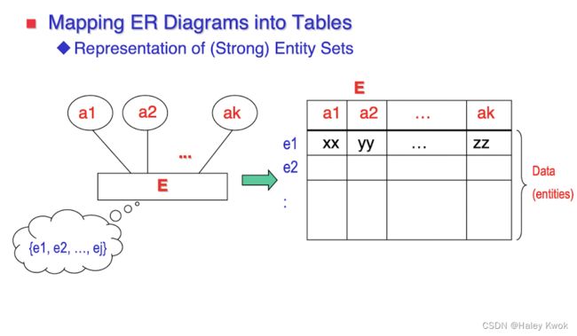
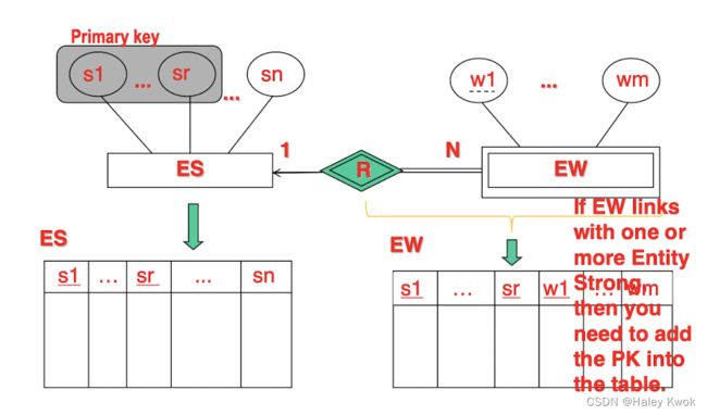
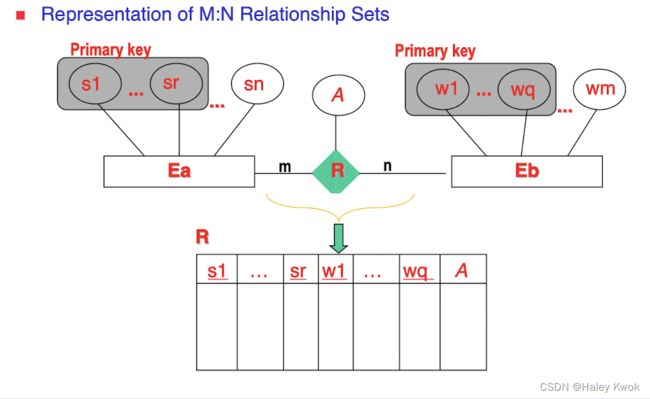
Method 2
(Primary Key#, Foreign Key*, Attribute, …, …)
9. Relationship of higher degree
The degree of relationship can be defined as the number of occurrences in one entity that is associated with the number of occurrences in another entity.
There is the three degree of relationship:
One-to-one (1:1)
One-to-many (1:M)
Many-to-many (M:N)
- One-to-one
In a one-to-one relationship, one occurrence of an entity relates to only one occurrence in another entity.
A one-to-one relationship rarely exists in practice.
For example: if an employee is allocated a company car then that car can only be driven by that employee.
Therefore, employee and company car have a one-to-one relationship.
- One-to-many
In a one-to-many relationship, one occurrence in an entity relates to many occurrences in another entity.
For example: An employee works in one department, but a department has many employees.
Therefore, department and employee have a one-to-many relationship.
- Many-to-many
In a many-to-many relationship, many occurrences in an entity relate to many occurrences in another entity.
Same as a one-to-one relationship, the many-to-many relationship rarely exists in practice.
For example: At the same time, an employee can work on several projects, and a project has a team of many employees.
Therefore, employee and project have a many-to-many relationship.
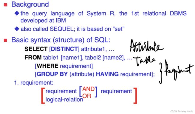
Chapter 3: SQL
Some of The Most Important SQL Commands
• SELECT - extracts data from a database
• UPDATE - updates data in a database
• DELETE - deletes data from a database
• INSERT INTO - inserts new data into a database
• CREATE DATABASE - creates a new database
• ALTER DATABASE - modifies a database
• CREATE TABLE - creates a new table
• ALTER TABLE - modifies a table
• DROP TABLE - deletes a table
• CREATE INDEX - creates an index (search key)
• DROP INDEX - deletes an index

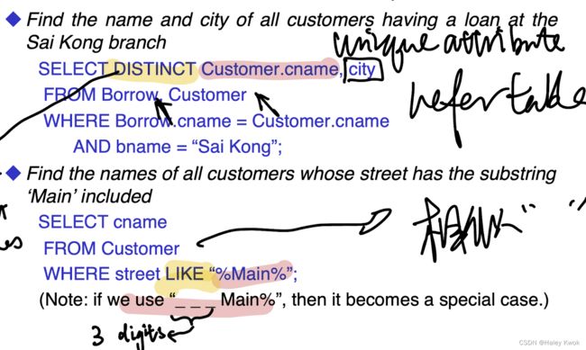
Examples
More than one attribute has the same name, therefore, you need to specify the name with '.'
You don’t have to use UNION???
SELECT DISTINCT Customer.cname, city
FROM Customer, Borrow
WHERE bname = 'Sai Kong'
AND Borrow.cname = Customer.cname;
You can see that you don’t have to join anything when you need to select two things, since they can be linked.
SELECT DATA (from bottom to top) SELECT IS THE COLUMN RESULT
SELECT column1, column2, ... -- the columns only exist in the output
FROM table_name;

SELECT CustomerName, City
FROM Customers;

SELECT *
FROM Customers;
1. DISTINCT
In a table, there may be a chance to exist a duplicate value and sometimes we want to retrieve only unique values. In such scenarios, SQL SELECT DISTINCT statement is used.
SELECT DISTINCT column1, column2, ...
FROM table_name;

SELECT DISTINCT home_town
FROM students
2. AND/OR/NOT
SELECT column1, column2, ...
FROM table_name
WHERE condition;

SELECT column1, column2, ...
FROM table_name
WHERE condition1 AND condition2 AND condition3 ...; #CAN BE ,

SELECT * FROM Customers
WHERE Country='Germany' AND City='Berlin';
SELECT column1, column2, ...
FROM table_name
WHERE condition1 OR condition2 OR condition3 ...;

SELECT * FROM Customers
WHERE City='Berlin' OR City='München';
SELECT column1, column2, ...
FROM table_name
WHERE NOT condition;

SELECT * FROM Customers
WHERE Country='Germany' AND (City='Berlin' OR City='München');
3. ORDER BY
SELECT column1, column2, ...
FROM table_name
ORDER BY column1, column2, ... ASC|DESC;
4. IS NULL/ IS NOT NULL
SELECT column_names
FROM table_name
WHERE column_name IS NULL;

SELECT column_names
FROM table_name
WHERE column_name IS NOT NULL;
5. TOP
SELECT TOP number|percent column_name(s)
FROM table_name
WHERE condition;

SELECT TOP 3 * FROM Customers;
SELECT TOP 50 PERCENT * FROM Customers;
6. MIN MAX
SELECT MIN|MAX(column_name)
FROM table_name
WHERE condition;
SELECT MIN(Price) AS SmallestPrice
FROM Products;
SELECT MAX(Price) AS LargestPrice
FROM Products;
7. COUNT/AVG/SUM
SELECT COUNT|AVG|SUM (column_name)
FROM table_name
WHERE condition;
8. LIKE
SELECT column1, column2, ...
FROM table_name
WHERE columnN LIKE pattern;

LIKE Operator	Description
WHERE CustomerName LIKE 'a%'	Finds any values that start with "a"
WHERE CustomerName LIKE '%a'	Finds any values that end with "a"
WHERE CustomerName LIKE '%or%'	Finds any values that have "or" in any position
WHERE CustomerName LIKE '_r%'	Finds any values that have "r" in the second position
WHERE CustomerName LIKE 'a_%'	Finds any values that start with "a" and are at least 2 characters in length
WHERE CustomerName LIKE 'a__%'	Finds any values that start with "a" and are at least 3 characters in length
WHERE ContactName LIKE 'a%o'	Finds any values that start with "a" and ends with "o"

Symbol	Description	Example
*	Represents zero or more characters	bl* finds bl, black, blue, and blob
?	Represents a single character	h?t finds hot, hat, and hit
[]	Represents any single character within the brackets	h[oa]t finds hot and hat, but not hit
!	Represents any character not in the brackets	h[!oa]t finds hit, but not hot and hat
-	Represents any single character within the specified range	c[a-b]t finds cat and cbt
'#'	Represents any single numeric character	2#5 finds 205, 215, 225, 235, 245, 255, 265, 275, 285, and 295
9. IN
SELECT column_name(s)
FROM table_name
WHERE column_name IN (value1, value2, ...);
#or
SELECT column_name(s)
FROM table_name
WHERE column_name IN (SELECT STATEMENT);
10. BETWEEN…AND/ NOT BETWEEN…AND
SELECT column_name(s)
FROM table_name
WHERE column_name BETWEEN value1 AND value2;

SELECT * FROM Products
WHERE Price NOT BETWEEN 10 AND 20;

SELECT * FROM Products
WHERE Price BETWEEN 10 AND 20
AND CategoryID NOT IN (1,2,3);

SELECT * FROM Products
WHERE ProductName BETWEEN 'Carnarvon Tigers' AND 'Mozzarella di Giovanni'
ORDER BY ProductName;
11. AS
Table

SELECT column_name AS alias_name
FROM table_name;

Column

SELECT column_name(s)
FROM table_name AS alias_name;

SELECT CustomerID AS ID, CustomerName AS Customer
FROM Customers;

SELECT CustomerName AS Customer, ContactName AS [Contact Person] #contain space need []
FROM Customers;

SELECT CustomerName, Address + ', ' + PostalCode + ' ' + City + ', ' + Country AS Address
FROM Customers;
12. ALL and ANY
ALL means that the condition will be true only if the operation is true for all values in the range.
is used with SELECT, WHERE and HAVING statements
SELECT column_name(s) FROM table1
UNION|ALL
SELECT column_name(s) FROM table2;
The following SQL statement lists the ProductName if ALL the records in the OrderDetails table has Quantity equal to 10. This will of course return FALSE because the Quantity column has many different values (not only the value of 10):
SELECT ProductName
FROM Products
WHERE ProductID = ALL
  (SELECT ProductID
  FROM OrderDetails
  WHERE Quantity = 10);
ANY means that the condition will be true if the operation is true for any of the values in the range.
The following SQL statement lists the ProductName if it finds ANY records in the OrderDetails table has Quantity larger than 99 (this will return TRUE because the Quantity column has some values larger than 99):
SELECT ProductName
FROM Products
WHERE ProductID = ANY
  (SELECT ProductID
  FROM OrderDetails
  WHERE Quantity = 10);
AGGREGATE
13. GROUP BY
The GROUP BY statement groups rows that have the same values into summary rows, like “find the number of customers in each country”.
The GROUP BY statement is often used with aggregate functions (COUNT(), MAX(), MIN(), SUM(), AVG()) to group the result-set by one or more columns.
Group by statement is used to group the rows that have the same value. Whereas Order by statement sort the result-set either in ascending or in descending order. … In select statement, it is always used before the order by keyword.
SELECT column_name(s)
FROM table_name
WHERE condition
GROUP BY column_name(s)
ORDER BY column_name(s);

SELECT COUNT(CustomerID), Country
FROM Customers
GROUP BY Country
ORDER BY COUNT(CustomerID) DESC;
-- MostRentBook: Correct
SELECT bookName, ISBN, author, bookCategory, SUM(bookRentNum)
FROM BOOK
GROUP BY bookName, ISBN, author, bookCategory
HAVING SUM(bookRentNum) >=
ALL(SELECT SUM(bookRentNum)
FROM book
GROUP BY ISBN);
SELECT bookName, ISBN, author, bookCategory, SUM(bookRentNum)
FROM book
GROUP BY bookName, ISBN, author, bookCategory, ISBN
HAVING (SUM(bookRentNum) >=
ALL(SELECT SUM(B.bookRentNum)
FROM book B
GROUP BY B.ISBN));


-- MostRentBook: Wrong
-- SELECT A.bookName, A.ISBN, A.author, A.bookCategory, SUM(A.bookRentNum)
-- FROM book A
-- GROUP BY A.ISBN
-- HAVING SUM(A.bookRentNum) >= ALL(SELECT SUM(B.bookRentNum) FROM book B GROUP BY B.ISBN)
14. HAVING (with aggregate functions only)
The HAVING clause was added to SQL because the WHERE keyword cannot be used with aggregate functions.
An aggregate function in SQL performs a calculation on multiple values and returns a single value. SQL provides many aggregate functions that include avg, count, sum, min, max, etc.
SELECT column_name(s)
FROM table_name
WHERE condition
GROUP BY column_name(s)
HAVING condition
ORDER BY column_name(s);

SELECT COUNT(CustomerID), Country
FROM Customers
GROUP BY Country
HAVING COUNT(CustomerID) > 5;
- ANY
The ANY and ALL operators allow you to perform a comparison between a single column value and a range of other values.
The ALL operator:
• returns a boolean value as a result
• returns TRUE if ALL of the subquery values meet the condition
• is used with SELECT, WHERE and HAVING statements
ALL means that the condition will be true only if the operation is true for all values in the range.
SELECT column_name(s)
FROM table_name
WHERE column_name operator ANY
  (SELECT column_name
  FROM table_name
  WHERE condition);
The following SQL statement lists the ProductName if it finds ANY records in the OrderDetails table has Quantity equal to 10 (this will return TRUE because the Quantity column has some values of 10):
SELECT ProductName
FROM Products
WHERE ProductID = ANY
  (SELECT ProductID
  FROM OrderDetails
  WHERE Quantity = 10);
The following SQL statement lists the ProductName if ALL the records in the OrderDetails table has Quantity equal to 10. This will of course return FALSE because the Quantity column has many different values (not only the value of 10):
SELECT ProductName
FROM Products
WHERE ProductID = ALL
  (SELECT ProductID
  FROM OrderDetails
  WHERE Quantity = 10);
JOIN
You can use NATURAL LEFT JOIN or LEFT JOIN ON to solve this problem. The difference between them is that NATURAL LEFT JOIN will automatically match the common columns between two tables, while LEFT JOIN ON requires you to specify the common columns.
-- Correct:
SELECT Person.FirstName, Person.LastName, Address.City, Address.State
FROM Person NATURAL LEFT JOIN Address;
SELECT firstName, lastName, city, state
FROM Person p LEFT JOIN Address a
ON p.personId = a.personId;
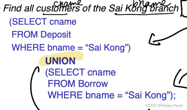
UNION
The UNION operator is used to combine the result-set of two or more SELECT statements.
Every SELECT statement within UNION must have the same number of columns
The columns must also have similar data types
The columns in every SELECT statement must also be in the same order
SELECT employee_id
FROM Employees
WHERE employee_id NOT IN (SELECT employee_id
                          FROM Salaries)
UNION
SELECT employee_id
FROM Salaries
WHERE employee_id NOT IN (SELECT employee_id
                          FROM Employees)
ORDER BY employee_id;
INSERT INTO DATA (from top to bottom)
INSERT INTO table_name (column1, column2, column3, ...)
VALUES (value1, value2, value3, ...);

UPDATE
UPDATE table_name
SET column1 = value1, column2 = value2, ...
WHERE condition;

***WARNING ALL DATA WOULD BE UPDATED AS Juan
UPDATE Customers
SET ContactName='Juan';

DELETE
1.
DELETE FROM table_name
WHERE condition;
2.
DELETE FROM table_name;


-TABLE
•	(INNER) JOIN: Returns records that have matching values in both tables
•	LEFT (OUTER) JOIN: Returns all records from the left table, and the matched records from the right table
•	RIGHT (OUTER) JOIN: Returns all records from the right table, and the matched records from the left table
•	FULL (OUTER) JOIN: Returns all records when there is a match in either left or right table


INNER\RIGHT\LEFT JOIN

SELECT column_name(s)
FROM table1
INNER JOIN table2
ON table1.column_name = table2.column_name;

SELECT Orders.OrderID, Customers.CustomerName, Orders.OrderDate
FROM Orders
INNER JOIN Customers ON Orders.CustomerID=Customers.CustomerID;

SELECT Orders.OrderID, Customers.CustomerName, Shippers.ShipperName
FROM ((Orders
INNER JOIN Customers ON Orders.CustomerID = Customers.CustomerID)
INNER JOIN Shippers ON Orders.ShipperID = Shippers.ShipperID);

FULL JOIN

SELECT column_name(s)
FROM table1
FULL OUTER JOIN table2
ON table1.column_name = table2.column_name
WHERE condition;

SELECT Customers.CustomerName, Orders.OrderID
FROM Customers
FULL OUTER JOIN Orders ON Customers.CustomerID=Orders.CustomerID
ORDER BY Customers.CustomerName;

SELECT

SELECT *
INTO newtable [IN externaldb]
FROM oldtable
WHERE condition;

INSERT INTO

INSERT INTO table2
SELECT * FROM table1
WHERE condition;


INSERT INTO Customers (CustomerName, City, Country)
SELECT SupplierName, City, Country FROM Suppliers;

CREATE
CREATE TABLE table_name (
    column1 datatype,
    column2 datatype,
    column3 datatype,
   ....
);

CREATE TABLE Persons (
    PersonID int,
    LastName varchar(255),
    FirstName varchar(255),
    Address varchar(255),
    City varchar(255)
);


CREATE TABLE Persons (
    ID int NOT NULL,
    LastName varchar(255) NOT NULL,
    FirstName varchar(255) NOT NULL,
    Age int
);

CREATE TABLE Persons (
    ID int NOT NULL UNIQUE,
    LastName varchar(255) NOT NULL,
    FirstName varchar(255),
    Age int
);

CREATE TABLE Persons (
    ID int NOT NULL PRIMARY KEY,
    LastName varchar(255) NOT NULL,
    FirstName varchar(255),
    Age int
);

DROP
DROP TABLE table_name;

ALTER TABLE – ADD/DROP Column
ALTER TABLE table_name
ADD column_name datatype;

ALTER TABLE Customers
ADD Email varchar(255);

ALTER TABLE table_name
DROP COLUMN column_name;

ALTER TABLE Customers
DROP COLUMN Email;

ALTER TABLE Persons
MODIFY Age int NOT NULL;

-DATABASE

CREATE DATABASE databasename;

DROP DATABASE databasename;

BACKUP DATABASE databasename
TO DISK = 'filepath';

CASE
SELECT OrderID, Quantity,
CASE
    WHEN Quantity > 30 THEN 'The quantity is greater than 30'
    WHEN Quantity = 30 THEN 'The quantity is 30'
    ELSE 'The quantity is under 30'
END AS QuantityText
FROM OrderDetails;


COMMENTS
--SELECT * FROM Customers;
SELECT * FROM Products;
Multi-line comments start with /* and end with */.
Any text between /* and */ will be ignored.
The following example uses a multi-line comment as an explanation:
/*Select all the columns
of all the records
in the Customers table:*/
SELECT * FROM Customers;
Lab Java
javac -cp ojdbc8.jar simpleApplication.java
java -cp ojdbc8.jar:. simpleApplication
Enter your username: "20060241d"
Enter your password: iyrhpast
2/11 Discussion
Memory consumption 100, 1000
The database will process the data faster than the processing side
TO_DATE
Can’t update sql without modify
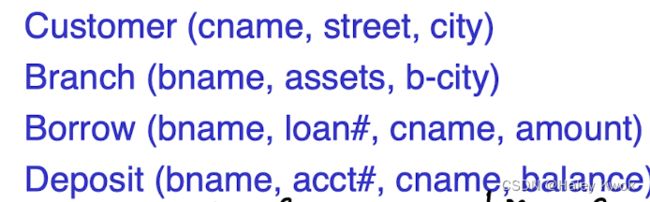
Chapter 4: Relational Model Concept
Relational model can represent as a table with columns and rows. Each row is known as a tuple. Each table of the column has a name or attribute.
Domain: It contains a set of atomic values that an attribute can take.
Attribute: It contains the name of a column in a particular table. Each attribute Ai must have a domain, dom(Ai)
Relational instance: In the relational database system, the relational instance is represented by a finite set of tuples. Relation instances do not have duplicate tuples.
Relational schema: A relational schema contains the name of the relation and name of all columns or attributes.
Relational key: In the relational key, each row has one or more attributes. It can identify the row in the relation uniquely.

In the given table, NAME, ROLL_NO, PHONE_NO, ADDRESS, and AGE are the attributes.
The instance of schema STUDENT has 5 tuples.
t3 =
Properties of Relations
Name of the relation is distinct from all other relations.
Each relation cell contains exactly one atomic (single) value
Each attribute contains a distinct name
Attribute domain has no significance
tuple has no duplicate value
Order of tuple can have a different sequence
1. Relational Algebra


1. Select Operation:
The select operation selects tuples that satisfy a given predicate.
It is denoted by sigma (σ).
Notation: σ p(r )
WHERE
where: σ is used for selection prediction
r is used for relation
p is used as a propositional logic formula which may use connectors like: AND OR and NOT. These relational can use as relational operators like =, ≠, ≥, <, >, ≤.
[Example]
LOAN Relation

Input: σ BRANCH_NAME=“perryride” (LOAN)
Output:


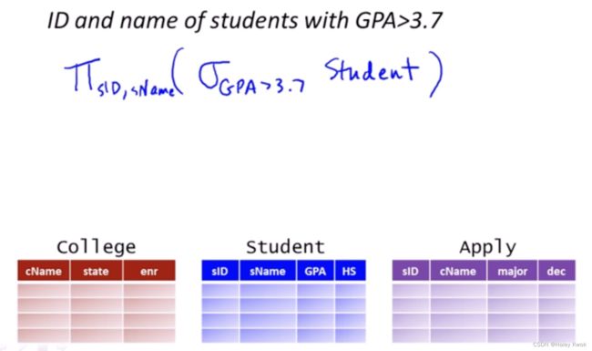
2. Project Operation
This operation shows the list of those attributes that we wish to appear in the result. Rest of the attributes are eliminated from the table.
It is denoted by ∏.
Notation: ∏ A1, A2, An (r )
FROM
Where A1, A2, A3 is used as an attribute name of relation r.
[Example]
CUSTOMER RELATION
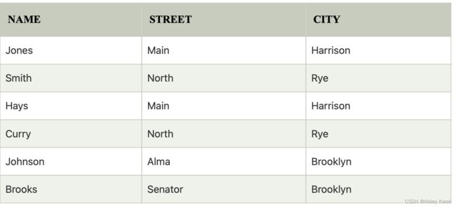
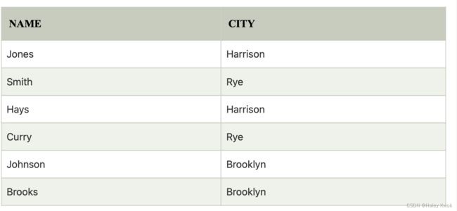
Input: ∏ NAME, CITY (CUSTOMER)
Output:

3. Union Operation (or):
Suppose there are two tuples R and S. The union operation contains all the tuples that are either in R or S or both in R & S.
It eliminates the duplicate tuples. It is denoted by ∪.
Notation: R ∪ S
A union operation must hold the following condition:
R and S must have the attribute of the same number.
Duplicate tuples are eliminated automatically.
[Example]
DEPOSITOR RELATION
BORROW RELATION
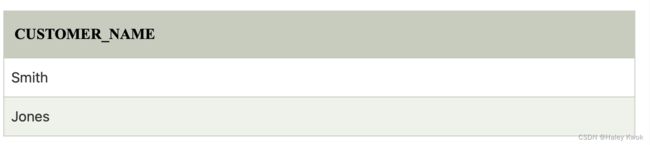
Input:
∏ CUSTOMER_NAME (BORROW) ∪ ∏ CUSTOMER_NAME (DEPOSITOR)
Output:

4. Set Intersection (and):
Suppose there are two tuples R and S. The set intersection operation contains all tuples that are in both R & S.
It is denoted by intersection ∩.
Notation: R ∩ S
Input:
∏ CUSTOMER_NAME (BORROW) ∩ ∏ CUSTOMER_NAME (DEPOSITOR)
Output:
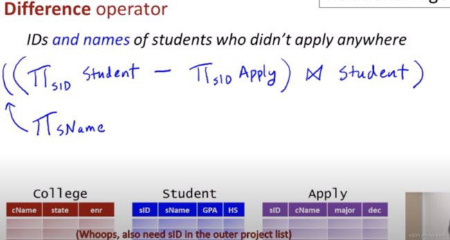
5. Set Difference:
Suppose there are two tuples R and S. The set intersection operation contains all tuples that are in R but not in S.
It is denoted by intersection minus (-).
Notation: R - S
[Example]
Using the above DEPOSITOR table and BORROW table
Input:
∏ CUSTOMER_NAME (BORROW) - ∏ CUSTOMER_NAME (DEPOSITOR)
Output:

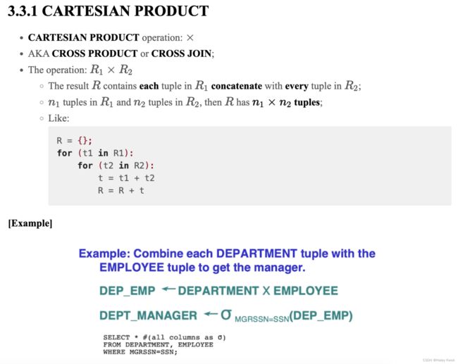
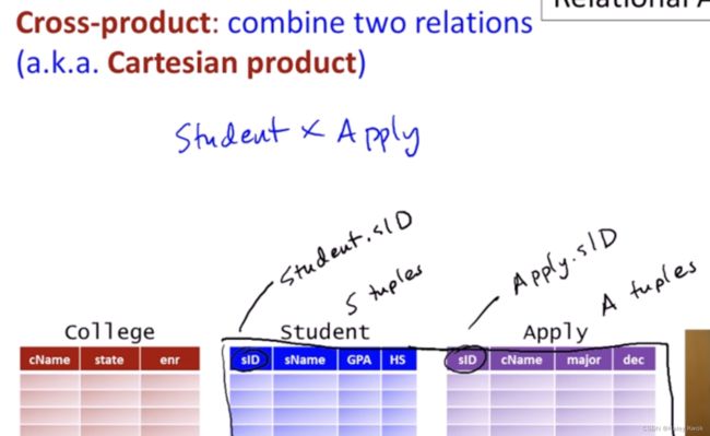
6. Cartesian product |><|
The Cartesian product is used to combine each row in one table with each row in the other table. It is also known as a cross product.
It is denoted by X.
Notation: E X D
[Example]
EMPLOYEE

DEPARTMENT
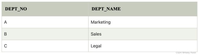
Input:
EMPLOYEE X DEPARTMENT
Output:

2. Join Operations:


A Join operation combines related tuples from different relations, if and only if a given join condition is satisfied. It is denoted by ⋈.
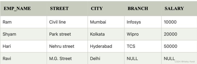
EMPLOYEE
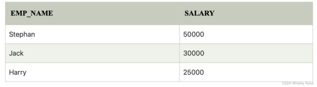
SALARY
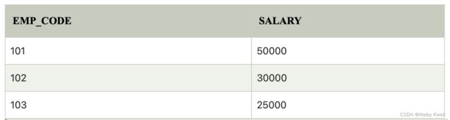
Operation: (EMPLOYEE ⋈ SALARY)

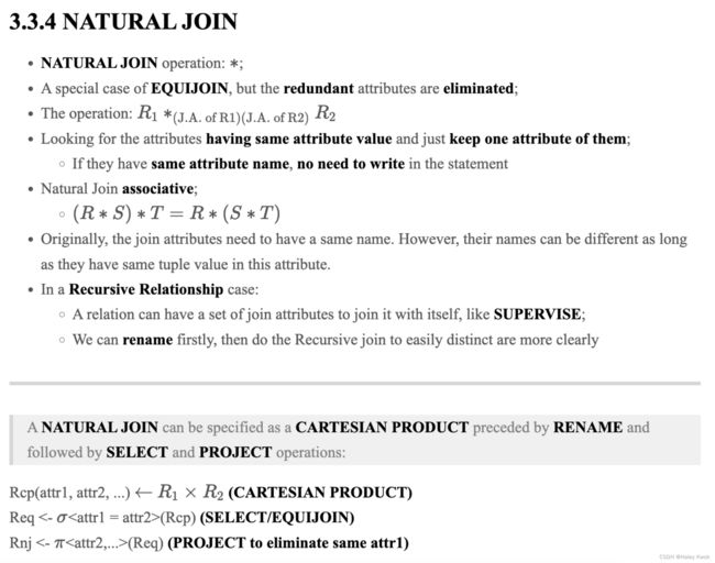
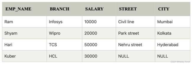
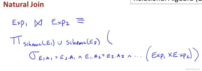
1. Natural Join

:
A natural join is the set of tuples of all combinations in R and S that are equal on their common attribute names.
It is denoted by ⋈.
Example: Let’s use the above EMPLOYEE table and SALARY table:
Input:
∏EMP_NAME, SALARY (EMPLOYEE ⋈ SALARY)
Output:

2. Outer Join:
The outer join operation is an extension of the join operation. It is used to deal with missing information.
Example:
EMPLOYEE

FACT_WORKERS
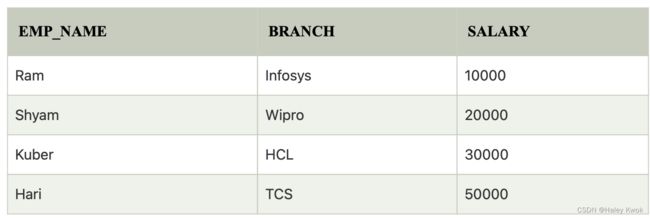
Input:
(EMPLOYEE ⋈ FACT_WORKERS)
Output:
An outer join is basically of three types:
Left outer join
Right outer join
Full outer join
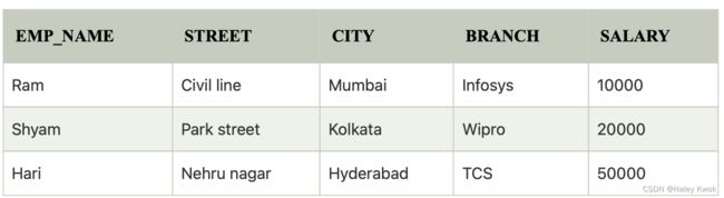
a. Left outer join:
Left outer join contains the set of tuples of all combinations in R and S that are equal on their common attribute names.
In the left outer join, tuples in R have no matching tuples in S.
It is denoted by ⟕.
Example: Using the above EMPLOYEE table and FACT_WORKERS table
Input:
EMPLOYEE ⟕ FACT_WORKERS
b. Right outer join:
EMPLOYEE ⟖ FACT_WORKERS
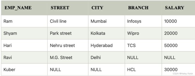
c. Full outer join:
In full outer join, tuples in R that have no matching tuples in S and tuples in S that have no matching tuples in R in their common attribute name
EMPLOYEE ⟗ FACT_WORKERS
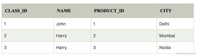
3. Equi join:
It is also known as an inner join. It is the most common join. It is based on matched data as per the equality condition. The equi join uses the comparison operator(=).
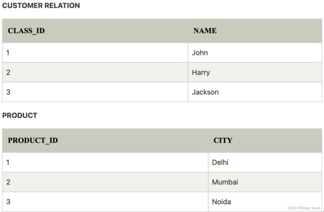
CUSTOMER ⋈ PRODUCT
Summary
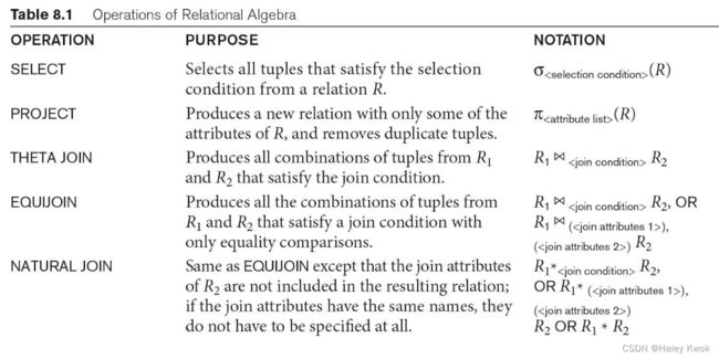
PRODUCT: distinct
EQUIJOIN: LIVES r1, LIVES r2, MANAGES m
NATURAL JOIN: LIVES, MANAGES
THINK FROM THE CONDITION, AND FINALLY FOR THE SELECT
SIGMA condition Rel.
PI cols… Rel.


You don’t have to = tow tables.attribute anymore!


Chapter 5: Integrity Constraints (ICs) and Normal Forms
Integrity constraints are a set of rules. It is used to maintain the quality of information.
Integrity constraints ensure that the data insertion, updating, and other processes have to be performed in such a way that data integrity is not affected.
Thus, integrity constraint is used to guard against accidental damage to the database.

1. Domain Constraint
Domain constraints can be defined as the definition of a valid set of values for an attribute.
The data type of domain includes string, character, integer, time, date, currency, etc. The value of the attribute must be available in the corresponding domain. It may also prohibit ‘null’ values of particular attributes.
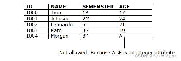
Number(6,2) -> 6 digits in total; and 2 digits after the decimal points
1234.56
2. Entity Integrity Constraint
The entity integrity constraint states that primary key value can't be null.
This is because the primary key value is used to identify individual rows in relation and if the primary key has a null value, then we can’t identify those rows.
A table can contain a null value other than the primary key field.

3. Referential Integrity Constraint
A referential integrity constraint is specified between two tables.
In the Referential integrity constraints, if a foreign key in Table 1 refers to the Primary Key of Table 2, then every value of the Foreign Key in Table 1 must be null or be available in Table 2.


4. Key Constraint
Keys are the entity set that is used to identify an entity within its entity set uniquely.
An entity set can have multiple keys, but out of which one key will be the primary key. A primary key can contain a unique and null value in the relational table.

Functional Dependency and Normal Forms
Functional Dependency (FD) is a particular kind of constraint that is on the set of “legal” relations n Formal definition:
The functional dependency is a relationship that exists between two attributes. It typically exists between the primary key and non-key attribute within a table.
Actually it implies that if you can find the non-key attribute, it may be easier for you to find out the primary key and candidate keys.
X → Y
The left side of FD is known as a determinant, the right side of the production is known as a dependent.
Assume we have an employee table with attributes: Emp_Id, Emp_Name, Emp_Address.
Here Emp_Id attribute can uniquely identify the Emp_Name attribute of employee table because if we know the Emp_Id, we can tell that employee name associated with it. We can say that Emp_Name is functionally dependent on Emp_Id.
Functional dependency can be written as:
Emp_Id → Emp_Name
Types of Functional Dependency
1. Trivial functional dependency
A → B has trivial functional dependency if B is a subset of A.
The following dependencies are also trivial like: A → A, B → B, AB -> A,…
2. Non-trivial functional dependency
A → B has a non-trivial functional dependency if B is not a subset of A.
When A intersection B is NULL, then A → B is called as complete non-trivial.
Inference Rules for FDs
1. Reflexive Rule (IR1)
In the reflexive rule, if Y is a subset of X, then X determines Y.
superkey and candidate key
If X ⊇ Y then X → Y
Example:
X = {a, b, c, d, e}
Y = {a, b, c}
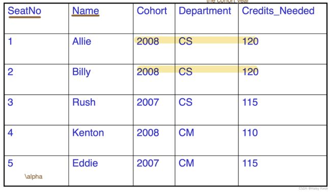
α \alpha α -> β \beta β
The Cohort AND Department -> Credits_Needed
SeatNo/ Name -> …
2. Augmentation Rule (IR2)
Commonly being ignored, but very important.
The augmentation is also called as a partial dependency. In augmentation, if X determines Y, then XZ determines YZ for any Z.
If X → Y then XZ → YZ (XZ stands for X U Z)
Example:
For R(ABCD), if A → B then AC → BC
3. Transitive Rule (IR3)
In the transitive rule, if X determines Y and Y determine Z, then X must also determine Z.
If X → Y and Y → Z then X → Z
4. Union Rule (IR4)
Union rule says, if X determines Y and X determines Z, then X must also determine Y and Z.
If X → Y and X → Z then X → YZ
Proof:
- X → Y (given)
- X → Z (given)
- X → XY (using IR2 on 1 by augmentation with X. Where XX = X)
- XY → YZ (using IR2 on 2 by augmentation with Y)
- X → YZ (using IR3 on 3 and 4)
5. Decomposition Rule (IR5)
Decomposition rule is also known as project rule. It is the reverse of union rule.
This Rule says, if X determines Y and Z, then X determines Y and X determines Z separately.
If X → YZ then X → Y and X → Z
Proof:
- X → YZ (given)
- YZ → Y (using IR1 Rule)
- X → Y (using IR3 on 1 and 2)
6. Pseudo transitive Rule (IR6)
In Pseudo transitive Rule, if X determines Y and YZ determines W, then XZ determines W.
If X → Y and YZ → W then XZ → W
Proof:
- X → Y (given)
- WY → Z (given)
- WX → WY (using IR2 on 1 by augmenting with W)
- WX → Z (using IR3 on 3 and 2)
Data modification anomalies can be categorized into three types:
Insertion Anomaly: Insertion Anomaly refers to when one cannot insert a new tuple into a relationship due to lack of data.
Deletion Anomaly: The delete anomaly refers to the situation where the deletion of data results in the unintended loss of some other important data.
Updatation Anomaly: The update anomaly is when an update of a single data value requires multiple rows of data to be updated.
Repetition, potential consistency, inability to represent, and loss of data
Types of Normal Forms:
Normalization works through a series of stages called Normal forms. The normal forms apply to individual relations. The relation is said to be in particular normal form if it satisfies constraints.
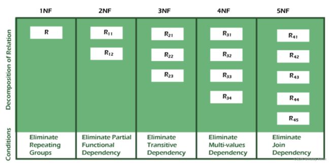

Normal Form Description
1NF
A relation is in 1NF if it contains an
atomic value. It states that an attribute of a table cannot hold multiple values. It must hold onlysingle-valued attribute.
Relation EMPLOYEE is not in 1NF because of multi-valued attribute EMP_PHONE.


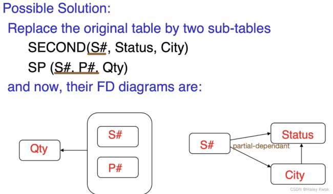
S# P# -> Qty
S# -> Status, City
City -> Status
, while Status and City is the non-key attribute, which forms partial relationship with the Primary key S#
Problems
- Insert Anomalies
Inability to represent certain information:
Eg, cannot enter “Supplier and City” information until Supplier supplies at least one part - Delete Anomalies
Deleting the “only tuple” for a supplier will destroy all the information about that supplier - Update Anomalies
“S# and City” could be redundantly represented for each P#, which may cause potential inconsistency when updating a tuple
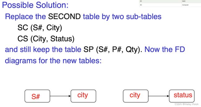
Solution
2NF
所有非关键字字段都由关键字段决定
不能部分依赖,就是说当一个表有组合主键时,其他非主键的字段必须完全依赖于主键。
No non-prime attribute is dependent on the proper subset of any candidate key of table
[Example]
for R1, F1 = {I->C, I->D, CD->N}
I is the only CK for RL, so no partial dependency in R1, hence satisfying 2NF.
but I->CD-> N is a transitive dependency, so violates 3NF, so R1 is 2NF

In the given table, non-prime attribute (Non-CK) TEACHER_AGE is dependent on TEACHER_ID which is a proper subset of a candidate key. That’s why it violates the rule for 2NF.


Update Problems: 1000 supplier live in Hong Kong and Hong Kong status. This pair information will be repeated for each of this 1000 supplier.
3NF (Good Design!)
Transitive functional dependencyof non-prime (non-CK) attribute on any super key should be removed.
[Example]
R(A,B,C,D,E)
F{A->B, BC->E, and ED->A}
CK: ABC, BCD, CDE
R is in the 3NF since all the attributes of R are ONLY key attributes.
所有非关键字字段都仅由关键字段决定
Super key in the table above:
{EMP_ID}, {EMP_ID, EMP_NAME}, {EMP_ID, EMP_NAME, EMP_ZIP}…so on
Candidate key: {EMP_ID}
Non-prime attributes: In the given table, all attributes except EMP_ID (CK) are non-prime.
Here, EMP_STATE & EMP_CITY dependent on EMP_ZIP and EMP_ZIP dependent on EMP_ID. The non-prime attributes (EMP_STATE, EMP_CITY) transitively dependent on super key(EMP_ID). It violates the rule of third normal form. 2NF ONLY
F{A,B,C,D,E}
A->C
C->DE
A->C->DE
That’s why we need to move the EMP_CITY and EMP_STATE to the new EMP_ZIP as a Primary key.

BCNF
A stronger definition of 3NF is known as Boyce Codd’s normal form. A relation R is in BCNF if and only if
every determinant (left-hand side of an FD) is a candidate key.

The combination of S#, P#

multiple candidate keys, and
these candidate keys are composite ones, and
they overlap on some common attribute
Chapter 6: File Organization and Indexing
File Organization
Data stored as magnetised areas on magnetic disk surfaces.
The block size B is fixed for each system. Typical block sizes range from B=512 bytes to B=4096 bytes.
Whole blocks are transferred between disk and main memory for processing.
Reading or writing a disk block is time consuming because of the seek time s and rotational delay (latency) rd
Double buffering can be used to speed up the transfer of contiguous disk blocks
A file is a sequence of records, where each record is a collection of data values.
Records are stored in disk blocks. The blocking factor bfr for a file is the (average) number of file records stored in a disk block.
A file can have fixed-length records or variable-length records.
File records can be unspanned (no record can span two blocks) -> a file with fixed-length records
or
spanned (a record can be stored in more than one block) -> a file with variable-length records
The physical disk blocks that are allocated to hold the records of a file can be contiguous, linked, or indexed
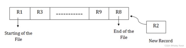
1. Unordered File
1.1 Pile File Method:
It is a quite simple method.
- To search for a record, a
linear searchthrough the file records is necessary. This requires reading and searching half the file blocks on the average, and is hence quite expensive. - Reading the records in order of a particular field requires sorting the file records.
- In this method, we store the record in a sequence, i.e., one after another.
- In case of updating or deleting of any record, the record will be searched in the memory blocks. When it is found, then it will be marked for deleting, and the new record is inserted.
- Here, the record will be inserted in the order in which they are inserted into tables. New records are inserted at the end of the file. Record insertion is quite efficient.
[Example]
Insertion of the new record:
Suppose we have four records R1, R3 and so on upto R9 and R8 in a sequence. Hence, records are nothing but a row in the table. Suppose we want to insert a new record R2 in the sequence, then it will be placed at the end of the file. Here, records are nothing but a row in any table.
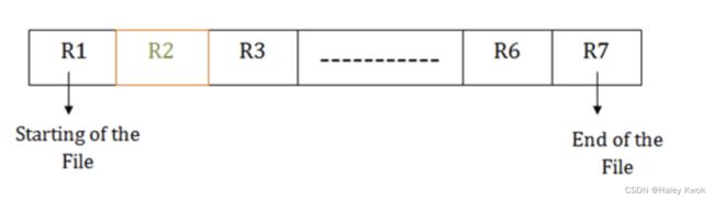
2. Ordered File (Sequential File Organization)
This method is the easiest method for file organization. In this method, files are stored sequentially.
2.1 Sorted File Method:
In this method, the new record is always inserted at the file’s end, and then it will sort the sequence in ascending or descending order. Sorting of records is based on any primary key or any other key.
In the case of modification of any record, it will update the record and then sort the file, and lastly, the updated record is placed in the right place.
Pros of sequential file organization
It contains a fast and efficient method for the huge amount of data.
In this method, files can be easily stored in cheaper storage mechanism like magnetic tapes.
It is simple in design.
It requires no much effort to store the data.
This method is used when most of the records have to be accessed like grade calculation of a student, generating the salary slip, etc.
This method is used for report generation or statistical calculations.
Cons of sequential file organization
It will waste time as we cannot jump on a particular record that is required but we have to move sequentially which takes our time.
Sorted file method takes more time and space for sorting the records.
[Example]
Insertion of the new record:
Suppose there is a preexisting sorted sequence of four records R1, R3 and so on upto R6 and R7. Suppose a new record R2 has to be inserted in the sequence, then it will be inserted at the end of the file, and then it will sort the sequence.
Binary Tree: Each node corresponds to a disk block; if the file has n blocks, the height of the tree will be l o g 2 n log_2n log2n

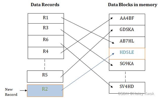
3. Heap Files (Unordered)
It is the simplest and most basic type of organization. It works with data blocks. In heap file organization, the records are inserted at the file’s end. When the records are inserted, it doesn’t require the sorting and ordering of records.
When the data block is full, the new record is stored in some other block. This new data block need not to be the very next data block, but it can select any data block in the memory to store new records. The heap file is also known as an unordered file.
Suppose we have five records R1, R3, R6, R4 and R5 in a heap and suppose we want to insert a new record R2 in a heap. If the data block 3 is full then it will be inserted in any of the database selected by the DBMS, let’s say data block 1.
Pros of Heap file organization
It is a very good method of file organization for bulk insertion. If there is a large number of data which needs to load into the database at a time, then this method is best suited.
In case of a small database, fetching and retrieving of records is faster than the sequential record.
Cons of Heap file organization
This method is inefficient for the large database because it takes time to search or modify the record. If we want to search, update or delete the data in heap file organization, then we need to traverse the data from staring of the file till we get the requested record.
This method is inefficient for large databases.
If the database is very large then searching, updating or deleting of record will be time-consuming because there is no sorting or ordering of records. In the heap file organization, we need to check all the data until we get the requested record.
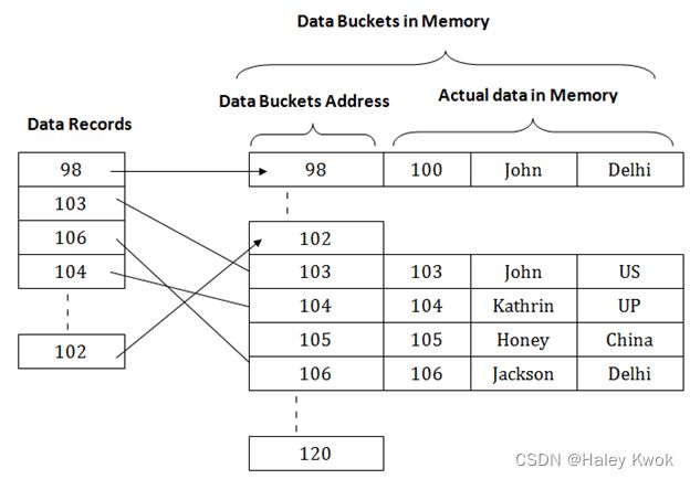
4. Hashed Files
The hash function h should distribute the records uniformly among the buckets. Otherwise, search time will increase because many overflow records will exist.
4.1 Static External Hashing
Hash File Organization uses the computation of hash function on some fields of the records. The hash function’s output determines the location of disk block where the records are to be placed.
One of the file fields is designated to be the hash key of the file. // Primary key itself as the address of the data block. That means each row whose address will be the same as a primary key stored in the data block.
The record with hash key value K is stored in bucket i, where i=h(K), and h is the hashing function.
Pros
- Search is very efficient on the hash key. In a huge database structure, it is very inefficient to search all the index values and reach the desired data. Hashing technique is used to calculate the direct location of a data record on the disk without using index structure. In this technique, data is stored at the data blocks whose address is generated by using the hashing function. The memory location where these records are stored is known as data bucket or data blocks. In this, a hash function can choose any of the column value to generate the address.
- When a record has to be received using the hash key columns, then the address is generated, and the whole record is retrieved using that address. In the same way, when a new record has to be inserted, then the address is generated using the hash key and record is directly inserted. The same process is applied in the case of delete and update.
- In this method, there is no effort for searching and sorting the entire file.
- In this method, each record will be stored randomly in the memory.
Cons
Fixed number of buckets M is a problem when the number of records in the file grows or shrinks
4.1.1 Collisions problem
Collisions occur when a new record hashes to a bucket that is
already full.
An overflow file is kept for storing such records;
overflow records that hash to each bucket can be linked together.
There are numerous methods for collision resolution, including the following: Open Addressing or Chaining
4.1.1.1 Opening Addressing: Linear Probing
When a hash function generates an address at which data is already stored, then the next bucket will be allocated to it. This mechanism is called as Linear Probing.
[Example]
try Bucket_id+1, Bucket_id+2, …
suppose R3 is a new address which needs to be inserted, the hash function generates address as 112 for R3. But the generated address is already full. So the system searches next available data bucket, 113 and assigns R3 to it.

4.1.1.2 Opening Addressing: Quadratic Probing
try Bucket_id+1, Bucket_id+4,…
3 + 4 = 7

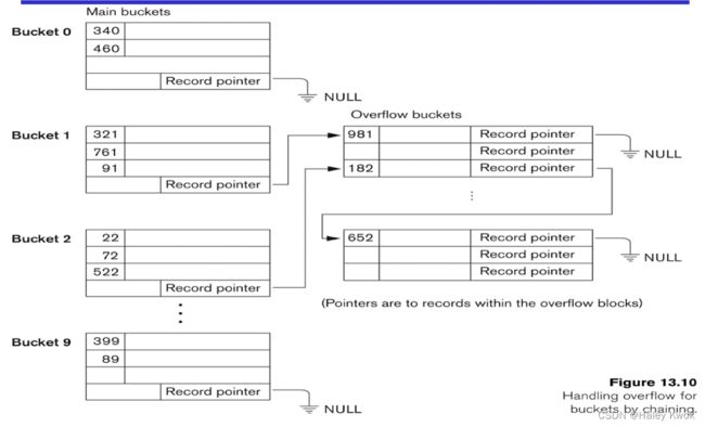
4.1.2 Overflow chaining/ Overflow handling
When buckets are full, then a new data bucket is allocated for the same hash result and is linked after the previous one. This mechanism is known as Overflow chaining.
For this method, various overflow locations are kept, usually by extending the array with a number of overflow positions.
In addition, a pointer field is added to each record location.
A collision is resolved by placing the new record in an unused overflow location and setting the pointer of the occupied hash address location to the address of that overflow location.
[Example]
Suppose R3 is a new address which needs to be inserted into the table, the hash function generates address as 110 for it. But this bucket is full to store the new data. In this case, a new bucket is inserted at the end of 110 buckets and is linked to it.

4.2 Dynamic And Extendible Hashing
The dynamic hashing method is used to overcome the problems of static hashing like bucket overflow. Dynamic and extendible hashing do not require an overflow area.
In this method, data buckets grow or shrink as the records increases or decreases. The directories can be stored on disk, and they expand or shrink dynamically. Directory entries point to the disk blocks that contain the stored records.
This method makes hashing dynamic, i.e., it allows insertion or deletion without resulting in poor performance.
Both dynamic and extendible hashing use the binary representation of the hash value h(K) in order to access a
directory.
In dynamic hashing the directory is a binary tree. In extendible hashing the directory is an array of size 2 d 2^d 2d where is called the global depth.
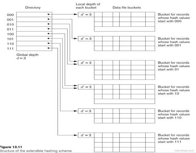
[Example]
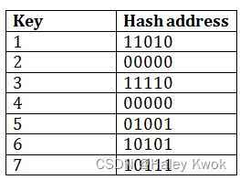
Insert key 9 with hash address 10001 into the above structure:
Since key 9 has hash address 10001, it must go into the first bucket. But bucket B1 is full, so it will get split.
The splitting will separate 5, 9 from 6 since last three bits of 5, 9 are 001, so it will go into bucket B1, and the last three bits of 6 are 101, so it will go into bucket B5.


Advantages of dynamic hashing
- In this method, the performance does not decrease as the data grows in the system. It simply increases the size of memory to accommodate the data.
- In this method, memory is well utilized as it grows and shrinks with the data. There will not be any unused memory lying. This method is good for the dynamic database where data grows and shrinks frequently.
Disadvantages of dynamic hashing
- In this method, if the data size increases then the bucket size is also increased. These addresses of data will be maintained in the bucket address table. This is because the data address will keep changing as buckets grow and shrink. If there is a huge increase in data, maintaining the bucket address table becomes tedious.
- In this case, the bucket overflow situation will also occur. But it might take little time to reach this situation than static hashing.
5. Indexing
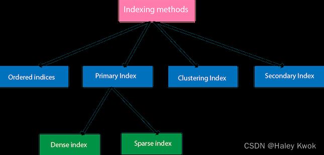
5.1 Ordered indices
The indices are usually sorted to make searching faster. The indices which are sorted are known as ordered indices.
[Example]
Suppose we have an employee table with thousands of record and each of which is 10 bytes long. If their IDs start with 1, 2, 3…and so on and we have to search student with ID-543.
In the case of a database with no index, we have to search the disk block from starting till it reaches 543. The DBMS will read the record after reading 54310=5430 bytes.
In the case of an index, we will search using indexes and the DBMS will read the record after reading 5422= 1084 bytes which are very less compared to the previous case.
5.1.1 Single level index/ Sparse indexing/ Primary index (Ordered)
Applicable conditions:
Primary index: applicable to a data file which is ordered on the key field (corresponding to the primary key of the corresponding relation), upon which the index is built, and it can be either a dense or non-dense index.
Query types supported by each:
Primary index: suitable for “one-record-at-a-time” search with a precise condition (such as given an id, find the corresponding employee); it can also be used to support “ordered read” according to the indexed field (eg, primary key).
是稀疏索引 仅指向每个块的地址
defined on ordered file
ordered on key field
1 index entry for each block (in data file)
index entry has key value for first record in block, i.e., block anchor
total number of entries in index is same as number of disk blocks
These primary keys are unique to each record and contain 1:1 relation between the records.
One form of an index:
a file of entries
一个主文件只可以有一个主索引,但可以有很多个辅助索引。
主索引建立在主码上,辅助索引建立在其他属性
主索引可以改变主文件的储存方式,(数据结构),但辅助索引不可以
5.1.1.1 Dense index
The dense index contains an index record for every search key value in the data file. It makes searching faster.
In this, the number of records in the index table is same as the number of records in the main table.
It needs more space to store index record itself. The index records have the search key and a pointer to the actual record on the disk.

5.1.1.2 Sparse index
In the data file, index record appears only for a few items. Each item points to a block.
In this, instead of pointing to each record in the main table, the index points to the records in the main table in a gap.
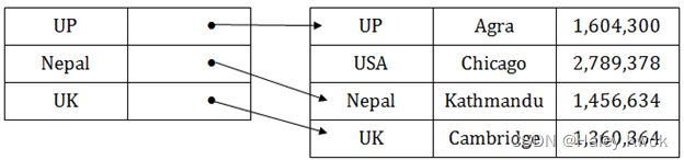
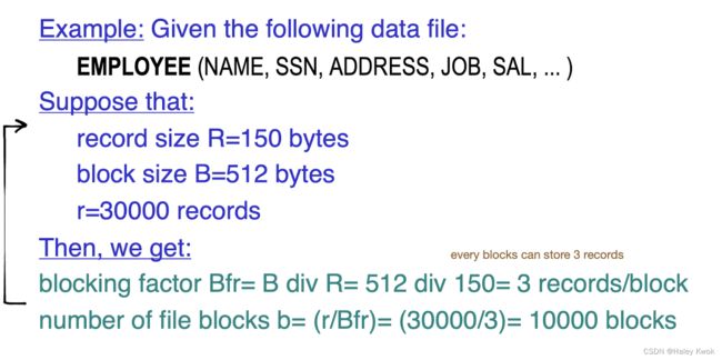
LINEAR SEARCH
blocking factor (Bfr) = 512/150 =3 records/book
number of file blocks b = 30000/3 = 10000 blocks
V.S.
BINARY SEARCH
index entry size = 9+7 = 16 bytes
index blocking factor Bfr = block size/ index entry size = 512/16 = 32 entries/ block
number of index block b = 30000/32 = 938 blocks
Binary search l o g 2 b log_2b log2b
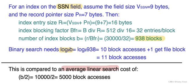

Advantages
In the sparse indexing, as the size of the table grows, the size of mapping also grows. These mappings are usually kept in the primary memory so that address fetch should be faster. Then the secondary memory searches the actual data based on the address got from mapping.
Disadvantages
If the mapping size grows then fetching the address itself becomes slower. In this case, the sparse index will not be efficient. To overcome this problem, secondary indexing is introduced.
5.2.1 Clustering index (Ordered)
Applicable conditions:
Clustering index: applicable to a data file which is ordered on a non-key field, upon which the index is built; it is normally a non-dense index.
Query types supported by each:
Clustering index: suitable for a “batch-at-a-time” search with an exact condition (eg, to list all employees of a given dept).
A clustered index can be defined as an ordered data file. Sometimes the index is created on non-primary key columns which may not be unique for each record.
In this case, to identify the record faster, we will group two or more columns to get the unique value and create index out of them.
The records which have similar characteristics are grouped, and indexes are created for these group.

[Example]
suppose a company contains several employees in each department. Suppose we use a clustering index, where all employees which belong to the same Dept_ID are considered within a single cluster, and index pointers point to the cluster as a whole. Here Dept_Id is a non-unique k

5.3.1 Secondary index (Non-ordered)
Applicable conditions:
Secondary index: applicable to a non-ordered data file, and the index is built either on a candidate key or a non-key field; it is always a dense index.
Query types supported by each:
Secondary index: suitable for either “ordered read” (if on a candidate key) or “batch-at-a-time” search (if on a non-key field), in both cases the data file is not required to be ordered.
辅助/二级索引
ordered file
2 fields:
1, same data fields as non ordering field
2, block pointer (not record pointer)
if 1 entry for each records, --> dense index
field value-block pointer -> blocks of records pointers -> data file
In the sparse indexing, as the size of the table grows, the size of mapping also grows. These mappings are usually kept in the primary memory so that address fetch should be faster. Then the secondary memory searches the actual data based on the address got from mapping. If the mapping size grows then fetching the address itself becomes slower. In this case, the sparse index will not be efficient. To overcome this problem, secondary indexing is introduced.
In secondary indexing, to reduce the size of mapping, another level of indexing is introduced. In this method, the huge range for the columns is selected initially so that the mapping size of the first level becomes small. Then each range is further divided into smaller ranges. The mapping of the first level is stored in the primary memory, so that address fetch is faster. The mapping of the second level and actual data are stored in the secondary memory (hard disk).

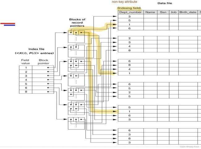
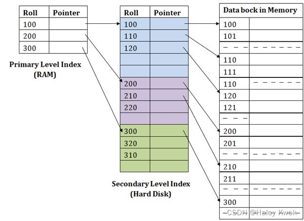
5.4.1 Multi-level index (primary, secondary, clustering)
Because a single-level index is an ordered file, we can level until all entries of the top level fit in one disk block
create a primary index to the index itself ; in this case, the original index file is called the first-level index and the index to the index is called the second-level index n We can repeat the process, creating a third, fourth, …, top
A single-level index is an ordered file, we can
level until all entries of the top level fit in one disk block
create a primary index to the index itself ; in this case, the original index file is called the first-level index and the index to the index is called the second-level index
A multi-level index can be created for any type of first- level index (primary, secondary, clustering) as long as the first-level index consists of more than one disk block
Such a multi-level index is a form of search tree; however, insertion and deletion of new index entries is a severe problem because every level of the index is an ordered file

Pros
A multi-level index can be created for any type of first-
level index (primary, secondary, clustering) as long as
the first-level index consists of more than one disk
block
Cons
Such a multi-level index is a form of search tree;
however, insertion and deletion of new index entries is
a severe problem because every level of the index is
an ordered file
5.4.2 Using B Trees and B+ Trees as Dynamic Multi-level Indexes
The B+ tree is a balanced binary search tree. It follows a multi-level index format.
B+ tree file organization is the advanced method of an indexed sequential access method. It uses a tree-like structure to store records in File.
It uses the same concept of key-index where the primary key is used to sort the records. For each primary key, the value of the index is generated and mapped with the record.
The B+ tree is similar to a binary search tree (BST), but it can have more than two children. In this method, all the records are stored only at the leaf node. Intermediate nodes act as a pointer to the leaf nodes. They do not contain any records.
Because of the insertion and deletion problem, most multi-level indexes use B tree or B + tree data structures, which leave space in each tree node (disk block) to allow for new index entries
- In B Tree and B+ Tree data structures, each node corresponds to a disk block
和B+树
B tree: 叶子节点处于同一级
B+:索引字段值重复出现
B:索引字段值仅出现一次
插入删除:
insertion into anode that is not full;
if full-> split into 2 nodes (maybe other tree levels)
deletion is efficient if more than half full
deletion-> half full, it will merge with neighbour
- Root Node
- Internal Node
- Leaf Node
Order of the tree is p = 4: 4 pointers
leaf order is: 3, means MAX three nodes (like boxes), but each node MUST keep between half-full and completely full, i.e., two in this case.
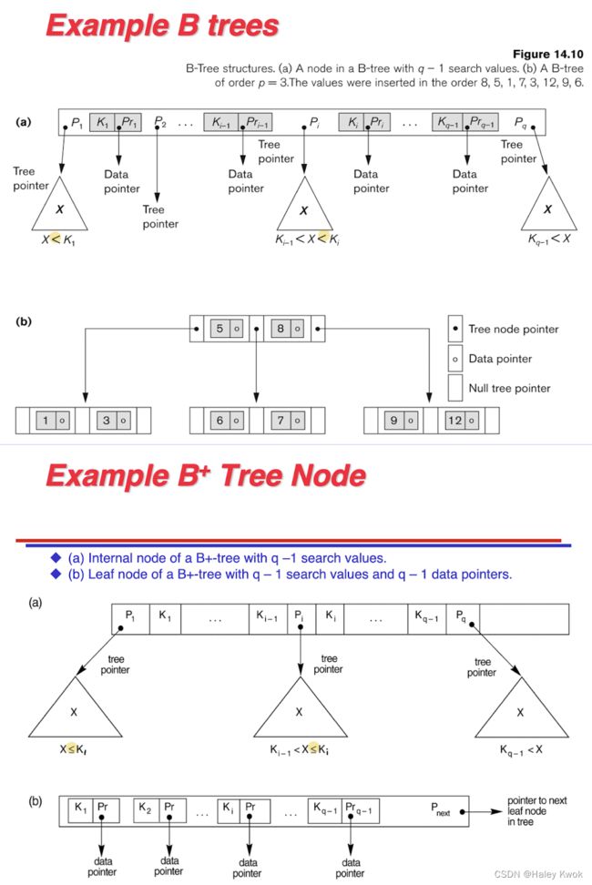
Insertion
- An insertion into a node that is not full is quite efficient; if a node is full the insertion causes a split into two nodes
- Splitting may propagate to other tree level
[Example]
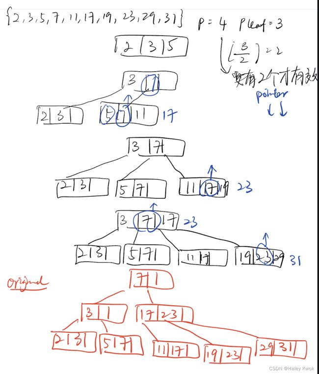
Delection
- A deletion is quite efficient if a node does not become less than half full
- If a deletion causes a node to become less than half full, it must be merged with neighboring nodes, where merge with the MAX value in the neighbouring nodes
- If there is one internal node left, we should delete the Root Node
[Example]
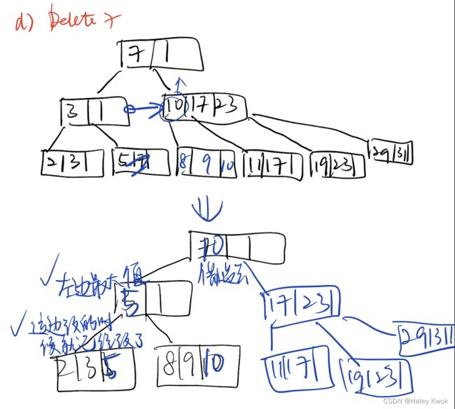

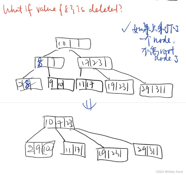
Pros of B+ tree file organization
- In this method, searching becomes very easy as all the records are stored only in the leaf nodes and sorted the sequential linked list. In the B+ tree, the leaf nodes are linked using a link list. Therefore, a B+ tree can support random access as well as sequential access.
- Traversing through the tree structure is easier and faster.
- The size of the B+ tree has no restrictions, so the number of records can increase or decrease and the B+ tree structure can also grow or shrink.
- It is a balanced tree structure, and any insert/update/delete does not affect the performance of tree.
Cons of B+ tree file organization
- This method is inefficient for the static method.
[Example]
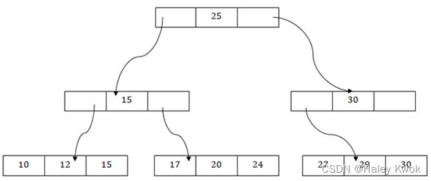
The above B+ tree shows that:
There is one root node of the tree, i.e., 25.
There is an intermediary layer with nodes. They do not store the actual record. They have only pointers to the leaf node.
The nodes to the left of the root node contain the prior value of the root and nodes to the right contain next value of the root, i.e., 15 and 30 respectively.
There is only one leaf node which has only values, i.e., 10, 12, 17, 20, 24, 27 and 29.
Searching for any record is easier as all the leaf nodes are balanced.
In this method, searching any record can be traversed through the single path and accessed easily.
[Example]
Insert 60

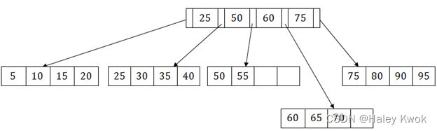
Denormalization
- The goal of normalization is to separate the logically related attributes into tables to minimize redundancy and thereby avoid the update anomalies that cause an extra processing overheard to maintain consistency of the database.
- The goal of denormalization is to improve the performance of frequently occurring queries and transactions. (Typically the designer adds to a table attributes that are needed for answering queries or producing reports so that a join with another table is avoided.)
Tuning:
The process of continuing to revise/adjust the physical database design by monitoring resource utilization as well as internal DBMS processing to reveal “bottlenecks” such as contention for the same data or devices.
Options to tuning indexes
Drop indexes or/and build new indexes
Change a non-clustered index to a clustered index (and vice
versa)
Rebuilding the index
A query with multiple selection conditions that are connected via OR may not encourage the query optimizer to use any index. -> Such a query may be split up and expressed as a union of queries, each with a condition on an attribute that causes an index to be used.
Apply the following transformations -> NOT condition may be transformed into a positive expression.
Embedded SELECT blocks may be replaced by joins. -> If an equality join is set up between two tables, the range predicate on the joining attribute set up in one table may be repeated for the other table WHERE conditions of SQL may be rewritten to utilize the indexes on multiple columns.
Chapter 7: Query Processing & Query Optimization
The process of choosing a suitable execution strategy for processing a query.
Two internal representations of a query:
Query Tree
Query Graph
1. Translating SQL Queries into Relational Algebra
2. Search Methods for Selection
Linear search (brute force)
Retrieve every record in the file;
Test whether its attribute values satisfy the selection condition.
Binary search
Condition: the selection condition involves an equality comparison on a
key attribute on which the file is ordered
An example is OP1 if SSN is the ordering attribute for the employee file.
Using a primary index or hash key to retrieve a single record
Condition: the selection condition involves an equality comparison on a key attribute with a primary index (or a hash key)
For example, SSN = 123456789 in OP1, we can use the primary index (or the hash key) to retrieve the record.
Using a primary index to retrieve multiple records
Condition: the comparison condition is >, ≥, <, or ≤ on a key field with a primary index
For example, dnumber > 5 in op2, we use the index to find the record satisfying the corresponding equality condition (dnumber = 5); then retrieve all subsequent records in the (ordered) file. For the condition dnumber < 5, retrieve all the preceding records.
Using a clustering index to retrieve multiple records
Condition: the selection condition involves an equality comparison on a nonkey attribute with a clustering index
for example, dno = 5 in op3, we use the clustering index to retrieve all the records satisfying the selection condition.
3. Calculation
1Let relations r1(A, B, C) and r2(C, D, E) have the following properties: r1 has 20,000 tuples, r2 has 45,000 tuples, 25 tuples of r1 fit on one block, and 30 tuples of r2 fit on one block. Estimate the number of block transfers and seeks required, using each of the following join strategies for r1 |X| r2:
r1 needs 800 blocks, and r2 needs 1500 blocks. Let us assume M pages of memory. If M > 800, the join can easily be done in 1500 + 800 disk accesses, using even plain nested-loop join. So we consider only the case where M ≤ 800 pages.
a. Nested-loop join
Using r1 as the outer relation we need 20000 ∗ 1500 + 800 = 30, 000, 800 disk accesses, if r2 is the outer relation we need 45000 ∗ 800+1500 = 36,001,500 disk accesses
b. Block nested-loop join
If r1 is the outer relation, we need ⌈ 800/ (M-1) ⌉ ∗ 1500 + 800 disk accesses,
if r2 is the outer relation we need ⌈ 1500/ (M-1) ⌉ ∗ 800 + 1500 disk accesses.
c. Merge join
Assuming that r1 and r2 are not initially sorted on the join key, the total sorting cost inclusive of the output is B s = 1500 ( 2 ⌈ l o g M − 1 ( 1500 / M ) ⌉ + 2 ) + 800 ( 2 ⌈ l o g M − 1 ( 800 / M ) ⌉ + 2 ) Bs = 1500(2⌈log_{M−1}(1500/M)⌉+2) + 800(2⌈log_{M−1}(800/M)⌉ + 2) Bs=1500(2⌈logM−1(1500/M)⌉+2)+800(2⌈logM−1(800/M)⌉+2) disk accesses. Assuming all tuples with the same value for the join attributes fit in memory, the total cost is Bs + 1500 + 800 disk accesses.
d. Hash join
Noted that there is overflow and non-overflow of the hash join; we assume there is no overflow. We also need to consider if there is recursive partitioning.
We assume no overflow occurs. Since r1 is smaller, we use it as the build relation and r2 as the probe relation. If M > 800/M, i.e. no need for recursive partitioning, then the cost is 3(1500+800) = 6900disk accesses, else the cost is 2 ( 1500 + 800 ⌈ l o g M − 1 ( 800 ) − 1 ⌉ + 1500 + 800 2(1500 + 800 ⌈log_{M−1}(800) − 1⌉ + 1500 + 800 2(1500+800⌈logM−1(800)−1⌉+1500+800 disk accesses.
Let relations R1(A,B,C) and R2(C,D,E) have the following properties:
R1 has 20,000 tuples, and 25 tuples of R1 fit on one block
R2 has 45,000 tuples, and 30 tuples of R2 fit on one block
Estimate the number of block accesses required, using each of the following join strategies for R1*R2:
-
Nested (inner-outer) loop [5 marks]
-
Sort-merge join [5 marks]
-
Hash-join [5 marks]
-
Using nested (inner-outer) loop strategy, for each tuple in R1, we must perform an access for each tuple in R2. This involves 20,000 x 45,000 = 900,000,000 accesses of tuples in R2. So when we include the 20,000 accesses to read R1, a total of 900,000,000 + 20,000 = 900,020,000 accesses are required.
-
Using sort-merge join strategy, if
(a) the relations are already sorted by the join attributes. In this case we read each block of R1 and R2 only once, therefore 20,000/25 + 45,000/30 = 2,300 accesses are required;
(b) the relations are not yet sorted, then we’ll need to sort the two tables first, so it requires (800Ln800 + 1500Ln1500) + (800+1500).
//the 1st parenthesis is for the two tables to sort, and the 2nd parenthesis is for the actual join. -
Using hash-join strategy, we need to first read both R1 and R2 in order to assign pointers to hash buckets, which entails reading 800 blocks (for R1) + 1500 blocks (for R2) = 2300 blocks. On the reasonable assumption that the hash buckets fit in main memory, no block accesses are incurred in creating or accessing the buckets. Each tuple is read once (at most) in the final computation of the join, incurring another 2300 blocks accesses. Therefore, totally 4600 blocks access is required.
//Note: although it can be worse than sort-merge join, it does NOT require the relations to be sorted.
4. Heuristic Algebraic Optimization Algorithm
Find the last names of employees born after 1957 who work on a project named ‘Aquarius’.
SELECT E.Lname
FROM EMPLOYEE E, WORKS_ON W, PROJECT P
WHERE P.Pname=‘Aquarius’ AND P.Pnumber=W.Pno AND E.Essn=W.Ssn
AND E.Bdate > ‘1957-12-31’;
FOLLOW THE SEQUENCE EMPLOYEE, WORKS_ON, PROJECT
= would be the restrictive, you can assume
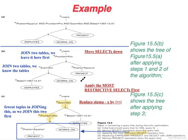
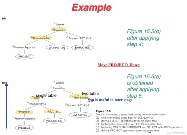
- order
- filter
- project
向上保留 向下删除
上面有什么就保留什么
Chapter 8: Transactions and Concurrency Control
Single-User System:
At most one user can use the system at one time.
Multiuser System:
Many users can access the system concurrently (at the same time).
Concurrency
Interleaved processing:
Concurrent execution of processes is interleaved in a single CPU.
Parallel processing:
Processes are concurrently executed in multiple CPUs
1. Transaction
The transaction is a set of logically related operation. It contains a group of tasks.
A transaction is an action or series of actions. It is performed by a single user to perform operations for accessing the contents of the database.
Read(X): Read operation is used to read the value of X from the database and stores it in a buffer in main memory. 1 2 3
Write(X): Write operation is used to write the value back to the database from the buffer. 1 2 3 4
- Find the address of the disk block that contains item X
- Copy that disk block into a buffer in main memory
- Copy item X form the program variable names X into its correct location in the buffer
- Store the updated block from the buffer back to disk
[Example]
- R(X);
- X = X - 500;
- W(X);
But it may be possible that because of the failure of hardware, software or power, etc. that transaction may fail before finished all the operations in the set.
To solve this problem, we have two important operations:
Commit: It is used to save the work done permanently.
Rollback: It is used to undo the work done.
1.1 Property of Transaction
- Atomicity
- It states that all operations of the transaction take place at once if not, the transaction is aborted.
- There is no midway, i.e., the transaction cannot occur partially. Each transaction is treated as one unit and either run to completion or is not executed at all.
Atomicity involves the following two operations:
Abort: If a transaction aborts then all the changes made are not visible.
Commit: If a transaction commits then all the changes made are visible.
[Example]
Let’s assume that following transaction T consisting of T1 and T2. A consists of Rs 600 and B consists of Rs 300. Transfer Rs 100 from account A to account B. After completion of the transaction, A consists of Rs 500 and B consists of Rs 400.
If the transaction T fails after the completion of transaction T1 but before completion of transaction T2, then the amount will be deducted from A but not added to B. This shows the inconsistent database state. In order to ensure correctness of database state, the transaction must be executed in entirety.
- Consistency
- The integrity constraints are maintained so that the database is consistent before and after the transaction.
- The execution of a transaction will leave a database in either its prior stable state or a new stable state.
- The consistent property of database states that every transaction sees a consistent database instance.
- The transaction is used to transform the database from one consistent state to another consistent state.
[Example]
The total amount must be maintained before or after the transaction.
Total before T occurs = 600+300=900
Total after T occurs= 500+400=900
Therefore, the database is consistent. In the case when T1 is completed but T2 fails, then inconsistency will occur.
- Isolation
- It shows that the data which is used at the time of execution of a transaction cannot be used by the second transaction until the first one is completed.
- In isolation, if the transaction T1 is being executed and using the data item X, then that data item can’t be accessed by any other transaction T2 until the transaction T1 ends.
- The concurrency control subsystem of the DBMS enforced the isolation property.
- Durability
- The durability property is used to indicate the performance of the database’s consistent state. It states that the transaction made the permanent changes.
- They cannot be lost by the erroneous operation of a faulty transaction or by the system failure. When a transaction is completed, then the database reaches a state known as the consistent state. That consistent state cannot be lost, even in the event of a system’s failure.
- The recovery subsystem of the DBMS has the responsibility of Durability property.
1.2 Transaction Status


- Active state
The active state is the first state of every transaction. In this state, the transaction is being executed.
[Example]
Insertion or deletion or updating a record is done here. But all the records are still not saved to the database.
- Partially committed
In the partially committed state, a transaction executes its final operation, but the data is still not saved to the database.
[Example]
In the total mark calculation example, a final display of the total marks step is executed in this state.
- Committed
Force writing a log
Before a transaction reaches its commit point, any portion of the
log that has not been written to the disk yet must now be written to the disk.
This process is called force-writing the log file before committing
a transaction.
A transaction is said to be in a committed state if it executes all its operations successfully. In this state, all the effects are now permanently saved on the database system.
- Failed state
If any of the checks made by the database recovery system fails, then the transaction is said to be in the failed state.
[Example]
In the example of total mark calculation, if the database is not able to fire a query to fetch the marks, then the transaction will fail to execute.
- Aborted/ Rollback
If any of the checks fail and the transaction has reached a failed state then the database recovery system will make sure that the database is in its previous consistent state. If not then it will abort or roll back the transaction to bring the database into a consistent state.
If the transaction fails in the middle of the transaction then before executing the transaction, all the executed transactions are rolled back to its consistent state.
After aborting the transaction, the database recovery module will select one of the two operations:
Re-start the transaction
Kill the transaction
2. Schedule
- Serial Schedule
The serial schedule is a type of schedule where one transaction is executed completely before starting another transaction. In the serial schedule, when the first transaction completes its cycle, then the next transaction is executed.
[Example]
Suppose there are two transactions T1 and T2 which have some operations. If it has no interleaving of operations, then there are the following two possible outcomes:
READ WRITE, READ WRITE, READ WRITE

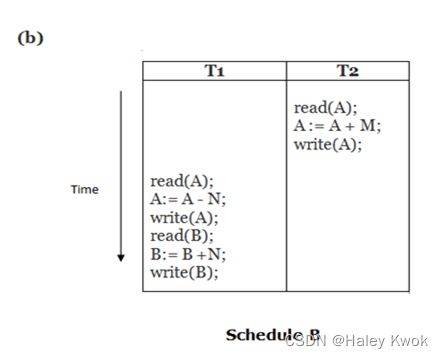
2. Non-serial Schedule
If interleaving of operations is allowed, then there will be non-serial schedule.
It contains many possible orders in which the system can execute the individual operations of the transactions.
[Example]
In the given figure © and (d), Schedule C and Schedule D are the non-serial schedules. It has interleaving of operations.
READ READ, WRITE READ, WRITE WRITE
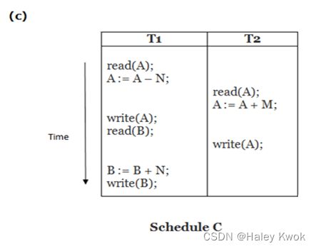

- Serializable Schedule
The serializability of schedules is used to find non-serial schedules that allow the transaction to execute concurrently without interfering with one another.
It identifies which schedules are correct when executions of the transaction have interleaving of their operations.
A non-serial schedule will be serializable if its result is equal to the result of its transactions executed serially.
Example
T1: w1(x), r1(y), w1(y)
T2: r2(x), r2(y), w2(y)
A possible schedule for T1 and T2:
w1(x), r2(x), r1(y), w1(y), r2(y), w2(y)
since it follows the original order
Is the following one a schedule?
r1(y), w1(y), r2(x), r2(y), w2(y), w1(x)
Nope, because w1(x) should be the first and now the order is changed.
3. Schedules Classified on Recoverability
A transaction may not execute completely due to a software issue, system crash or hardware failure. In that case, the failed transaction has to be rollback. But some other transaction may also have used value produced by the failed transaction. So we also have to rollback those transactions.
Cascaded rollback:
- A single failure leads to a series of rollback
- All uncommitted transactions that read an item from a failed transaction must be rolled back.
3.1 Non-recoverable schedule
non-recoverable schedule: The schedule will be irrecoverable if
- Tj reads the updated value of Ti
- Tj committed before Ti commit.
Write (A), Read (A)

The above table 1 shows a schedule which has two transactions. T1 reads and writes the value of A and that value is read and written by T2. T2 commits but later on, T1 fails. Due to the failure, we have to rollback T1. T2 should also be rollback because it reads the value written by T1, but T2 can’t be rollback because it already committed.
3.2 Recoverable schedule with cascaded rollback
Recoverable with cascaded rollback: The schedule will be recoverable with cascaded rollback if
- Tj reads the updated value of Ti
- Commit of Tj is delayed till commit of Ti.
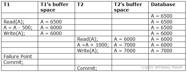
The above table 2 shows a schedule with two transactions. Transaction T1 reads and writes A, and that value is read and written by transaction T2. But later on, T1 fails. Due to this, we have to rollback T1. T2 should be rollback because T2 has read the value written by T1. As it has not committed before T1 commits so we can rollback transaction T2 as well. So it is recoverable with cascaded rollback.
3.3 Cascadeless schedule
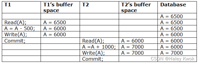
The above Table 3 shows a schedule with two transactions.
- Transaction T1 reads and write A and commits
- value is read and written by T2.
Every transaction reads only the items that are written by committed transactions.
In other words,
- Before Ti reads an item written by Tj
- Tj is already committed
3.4 Strict schedules
A schedule in which a transaction can neither read nor write an item X until the last transaction that wrote X has committed
Example
S: w1(X,5); w2(X,8); a1 (T1 aborts);
• Initially, X=9
• T1 writes a value 5 for X (keeping 9 as “before image”)
• T2 writes a value 8 for X (keeping 5 as “before image”)
• Then T1 aborts
Cascadeless
If the system restore according to the “before image” kept in T1, then 9 will be the value for X now, which means, the effect of T2 is lost
-> it does not violate the cascade less since there is no read here, but there is lost update problem
Strict
w2 can not happen until T1 commits
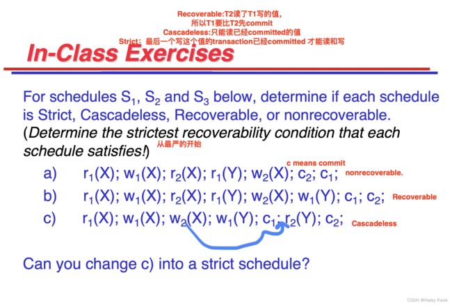
4. Schedules Classified on Serializability
4.1 Conflict Serializable Schedule
- A schedule is called conflict serializability if after swapping of non-conflicting operations, it can transform into a serial schedule.
- The schedule will be a conflict serializable if it is conflict equivalent (one can be transformed to another by swapping non-conflicting operations) to a serial schedule.
** conflict equivalent -> a serial schedule -> conflict serialisable
In short, it means there is no cycle and the -> can interpret others in the precedence graph, shown in Example.**
The two operations become conflicting if all conditions satisfy:
- Both belong to separate transactions.
- They have the same data item.
- They contain at least one write operation.
[Example]
Swapping is possible only if S1 and S2 are logically equal.
Here, S1 = S2. That means it is non-conflict.

Here, S1 ≠ S2. That means it is conflict.

4.2 Conflict Equivalent
In the conflict equivalent, one can be transformed to another by swapping non-conflicting operations. In the given example, S2 is conflict equivalent to S1 (S1 can be converted to S2 by swapping non-conflicting operations).
Two schedules are said to be conflict equivalent if and only if:
- They contain the same set of the transaction.
- If each pair of conflict operations are ordered in the same way.
[Example]
Schedule S2 is a serial schedule because, in this, all operations of T1 are performed before starting any operation of T2. Schedule S1 can be transformed into a serial schedule by swapping non-conflicting operations of S1.

After swapping of non-conflict operations, the schedule S1 becomes:
Since, S1 is conflict serializable.
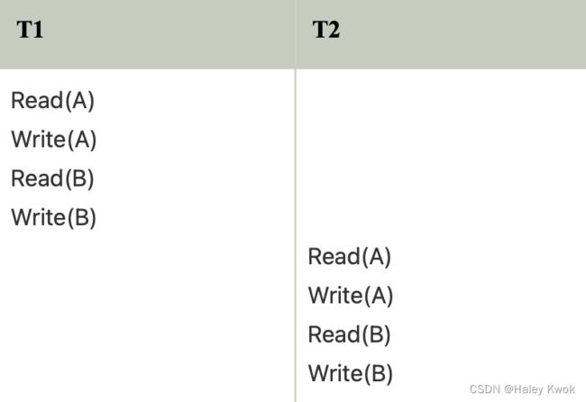
Conflict Equivalent
S1 and S2 are all WRITE READ
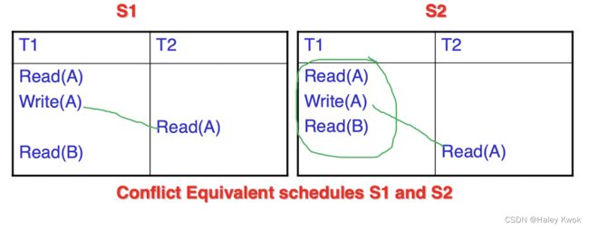
Not-Conflict Equivalent
This one is READ WRITE
READ A
READ A
WRITE A
READ B
4.3 Result equivalent
Two schedules are called result equivalent if they produce the same final state of the database.
Being serializable is not the same as being serial
Being serializable implies that the schedule is a correct schedule.
It will leave the database in a consistent state. The interleaving is appropriate and will result in a state as if the transactions were serially executed, yet will achieve efficiency due to concurrent execution.
5. Test of Serializability
Write Read
Read Write
Write Write
X READ READ
Create a node Ti → Tj if Ti executes write (Q) before Tj executes read (Q).
Create a node Ti → Tj if Ti executes read (Q) before Tj executes write (Q).
Create a node Ti → Tj if Ti executes write (Q) before Tj executes write (Q).
** 1. READ AND WRITE is a pair so with the same data you can ignore it, which means if the READ AND WRITE appears consecutively, you just use the WRITE to find the conflicting pairs
2. X READ READ **
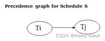
- If a precedence graph contains a single edge Ti → Tj, then all the instructions of Ti are executed before the first instruction of Tj is executed.
| precedence graph for schedule S contains a cycle | precedence graph for schedule S has no cycle |
|---|---|
| S is non-serializable | S is serializable |
5.1 Non-serializable schedule
[Example for Schedule S being non-serializable]
Read(A): In T1, no subsequent writes to A, so no new edges
Read(B): In T2, no subsequent writes to B, so no new edges
Read©: In T3, no subsequent writes to C, so no new edges
Write(B): B is subsequently read by T3, so add edge T2 → T3
Write©: C is subsequently read by T1, so add edge T3 → T1
Write(A): A is subsequently read by T2, so add edge T1 → T2
Write(A): In T2, no subsequent reads to A, so no new edges
Write©: In T1, no subsequent reads to C, so no new edges
Write(B): In T3, no subsequent reads to B, so no new edges


5.2 Serializable schedule
A schedule S is serializable if it is equivalent to some serial schedule of the same transactions.
[Example for Schedule S being serializable]
Read(A): In T4,no subsequent writes to A, so no new edges
Read(C ): In T4, no subsequent writes to C, so no new edges
Write(A): A is subsequently read by T5, so add edge T4 → T5
Read(B): In T5, no subsequent writes to B, so no new edges
Write(C ): C is subsequently read by T6, so add edge T4 → T6
Write(B): B is subsequently read by T6, so add edge T5 → T6
Write(C ): In T6, no subsequent reads to C, so no new edges
Write(A): In T5, no subsequent reads to A, so no new edges
Write(B): In T6, no subsequent reads to B, so no new edges
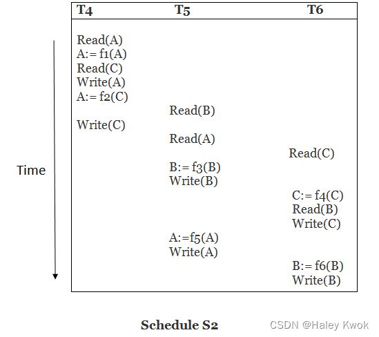
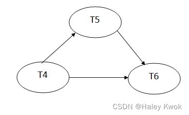
Example
STEP1: Based on the conflicting pair, we can produce the precedence graph
Write Read
Read Write
Write Write
X READ READ
Create a node Ti → Tj if Ti executes write (Q) before Tj executes read (Q).
Create a node Ti → Tj if Ti executes read (Q) before Tj executes write (Q).
Create a node Ti → Tj if Ti executes write (Q) before Tj executes write (Q).
** 1. READ AND WRITE is a pair so with the same data you can ignore it, which means if the READ AND WRITE appears consecutively, you just use the WRITE to find the conflicting pairs
2. X READ READ **

STEP2: we can draw the precedence graph to determine if it is,
** conflict equivalent -> a serial schedule -> conflict serialisable
In short, it means there is no cycle and the -> can interpret others in the precedence graph, shown in Example.**

STEP3: we can conclude that if we would like to make it serialisable, by changing the order

STEP1

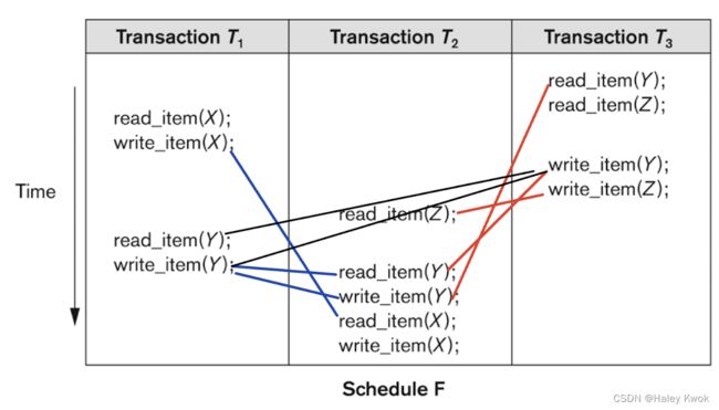
STEP2

Which of the following schedules is (conflict) serializable? For each serializable schedule, determine the equivalent serial schedules.
a) r1(X); r3(X); w1(X); r2(X); w3(X);
b) r1 (X); r 3 (X); w 3 (X); w 1 (X); r 2 (X);
c) r3 (X); r2 (X); w 3 (X); r1 (X); w1(X);
–
NOT YET MENTIONED IN TGE LECTURE
View Serializability
conflict serializable can be view serializable, view equivalent to a serial schedule.
The view serializable which does not conflict serializable contains blind writes.
View Equivalent
Two schedules S1 and S2 are said to be view equivalent if they satisfy the following conditions:
- Initial Read
An initial read of both schedules must be the same. Suppose two schedule S1 and S2. In schedule S1, if a transaction T1 is reading the data item A, then in S2, transaction T1 should also read A.
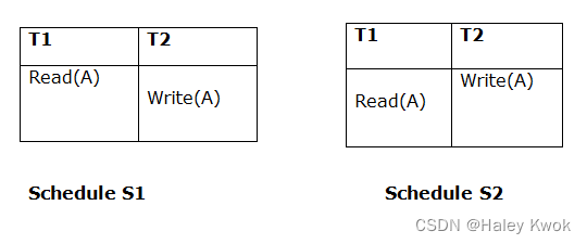
Above two schedules are view equivalent because Initial read operation in S1 is done by T1 and in S2 it is also done by T1.
- Updated Read
In schedule S1, if Ti is reading A which is updated by Tj then in S2 also, Ti should read A which is updated by Tj.
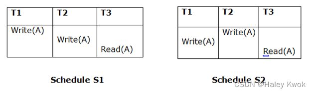
Above two schedules are not view equal because, in S1, T3 is reading A updated by T2 and in S2, T3 is reading A updated by T1.
- Final Write
A final write must be the same between both the schedules. In schedule S1, if a transaction T1 updates A at last then in S2, final writes operations should also be done by T1.
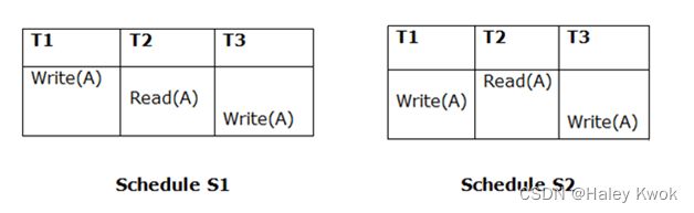
Above two schedules is view equal because Final write operation in S1 is done by T3 and in S2, the final write operation is also done by T3.
[Example]
Schedule S:
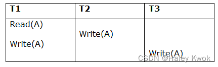
With 3 transactions, the total number of possible schedule
= 3! = 6
S1 =
S2 =
S3 =
S4 =
S5 =
S6 =
Taking first schedule S1:

Step 1: Initial Read
The initial read operation in S is done by T1 and in S1, it is also done by T1.
Step 2: final updation on data items
In both schedules S and S1, there is no read except the initial read that’s why we don’t need to check that condition.
Step 3: Final Write
The final write operation in S is done by T3 and in S1, it is also done by T3. So, S and S1 are view Equivalent.
The first schedule S1 satisfies all three conditions, so we don’t need to check another schedule.
Hence, view equivalent serial schedule is:
T1 → T2 → T3
–
Failure Classification
1. Transaction failure
The transaction failure occurs when it fails to execute or when it reaches a point from where it can’t go any further. If a few transaction or process is hurt, then this is called as transaction failure.
Reasons for a transaction failure could be:
- Logical errors: If a transaction cannot complete due to some code error or an internal error condition, then the logical error occurs.
- Syntax error: It occurs where the DBMS itself terminates an active transaction because the database system is not able to execute it. For example, The system aborts an active transaction because it violates serializability or because several transactions, in case of deadlock or resource unavailability.
2. System Crash
- System failure can occur due to power failure or other hardware or software failure.
Example: Operating system error.
Fail-stop assumption: In the system crash, non-volatile storage is assumed not to be corrupted.
3. Disk Failure
-
It occurs where hard-disk drives or storage drives used to fail frequently. It was a common problem in the early days of technology evolution.
-
Disk failure occurs due to the formation of bad sectors, disk head crash, and unreachability to the disk or any other failure, which destroy all or part of disk storage.
Log-Based Recovery
- The log is a sequence of records. Log of each transaction is maintained in some stable storage so that if any failure occurs, then it can be recovered from there.
- If any operation is performed on the database, then it will be recorded in the log.
- But the process of storing the logs should be done before the actual transaction is applied in the database.
[Example]
Let’s assume there is a transaction to modify the City of a student. The following logs are written for this transaction.
When the transaction is initiated, then it writes ‘start’ log.
When the transaction modifies the City from ‘Noida’ to ‘Bangalore’, then another log is written to the file.
When the transaction is finished, then it writes another log to indicate the end of the transaction.
There are two approaches to modify the database:
- Deferred database modification:
The deferred modification technique occurs if the transaction does not modify the database until it has committed.
In this method, all the logs are created and stored in the stable storage, and the database is updated when a transaction commits.
- Immediate database modification:
The Immediate modification technique occurs if database modification occurs while the transaction is still active.
In this technique, the database is modified immediately after every operation. It follows an actual database modification.
Recovery using Log records
When the system is crashed, then the system consults the log to find which transactions need to be undone and which need to be redone.
If the log contains the record
If log contains record
Checkpoint
- The checkpoint is a type of mechanism where all the previous logs are removed from the system and permanently stored in the storage disk.
- The checkpoint is like a bookmark. While the execution of the transaction, such checkpoints are marked, and the transaction is executed then using the steps of the transaction, the log files will be created.
- When it reaches to the checkpoint, then the transaction will be updated into the database, and till that point, the entire log file will be removed from the file. Then the log file is updated with the new step of transaction till next checkpoint and so on.
- The checkpoint is used to declare a point before which the DBMS was in the consistent state, and all transactions were committed.
Recovery using Checkpoint
In the following manner, a recovery system recovers the database from this failure:
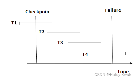
The recovery system reads log files from the end to start. It reads log files from T4 to T1.
Recovery system maintains two lists, a redo-list, and an undo-list.
The transaction is put into redo state if the recovery system sees a log with
[Example]
In the log file, transaction T2 and T3 will have
The transaction is put into undo state if the recovery system sees a log with
[Example]
Transaction T4 will have
Deadlock in DBMS
A deadlock is a condition where two or more transactions are waiting indefinitely for one another to give up locks. Deadlock is said to be one of the most feared complications in DBMS as no task ever gets finished and is in waiting state forever.
[Example]
In the student table, transaction T1 holds a lock on some rows and needs to update some rows in the grade table. Simultaneously, transaction T2 holds locks on some rows in the grade table and needs to update the rows in the Student table held by Transaction T1.
Now, the main problem arises. Now Transaction T1 is waiting for T2 to release its lock and similarly, transaction T2 is waiting for T1 to release its lock. All activities come to a halt state and remain at a standstill, where they are mutually waiting for each other. It will remain in a standstill until the DBMS detects the deadlock and aborts one of the transactions.

1. Deadlock Avoidance
When a database is stuck in a deadlock state, then it is better to avoid the database rather than aborting or restating the database. This is a waste of time and resource.
Deadlock avoidance mechanism is used to detect any deadlock situation in advance.
| larger database | smaller database |
|---|---|
| deadlock prevention | wait for graph |
2. Deadlock Detection
In a database, when a transaction waits indefinitely to obtain a lock, then the DBMS should detect whether the transaction is involved in a deadlock or not. The lock manager maintains a Wait for the graph to detect the deadlock cycle in the database.
3. Wait for Graph
This is the suitable method for deadlock detection. In this method, a graph is created based on the transaction and their lock. If the created graph has a cycle or closed loop, then there is a deadlock.
The wait for the graph is maintained by the system for every transaction which is waiting for some data held by the others. The system keeps checking the graph if there is any cycle in the graph.
The wait for a graph for the above scenario is shown below:
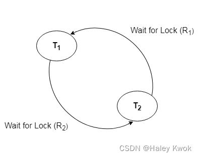
Deadlock Prevention
Deadlock prevention method is suitable for a large database. If the resources are allocated in such a way that deadlock never occurs, then the deadlock can be prevented.
The Database management system analyzes the operations of the transaction whether they can create a deadlock situation or not. If they do, then the DBMS never allowed that transaction to be executed.
1. Wait-Die scheme
In this scheme, if a transaction requests for a resource which is already held with a conflicting lock by another transaction then the DBMS simply checks the timestamp of both transactions. It allows the older transaction to wait until the resource is available for execution.
[Example]
Let’s assume there are two transactions Ti and Tj and let TS(T) is a timestamp of any transaction T. If T2 holds a lock by some other transaction and T1 is requesting for resources held by T2 then the following actions are performed by DBMS:
- Check if TS(Ti) < TS(Tj) - If Ti is the older transaction and Tj has held some resource, then Ti is allowed to wait until the data-item is available for execution. That means if the older transaction is waiting for a resource which is locked by the younger transaction, then the older transaction is allowed to wait for resource until it is available.
- Check if TS(Ti) < TS(Tj) - If Ti is older transaction and has held some resource and if Tj is waiting for it, then Tj is killed and restarted later with the random delay but with the same timestamp.
2. Wound wait scheme
| resource held by older transaction | resource held by younger transaction |
|---|---|
| younger transaction is asked to wait until older releases it | forces younger one to kill the transaction and release the resource. After the minute delay, the younger transaction is restarted but with the same timestamp. |
Chapter 8: DBMS Concurrency Control
Concurrency Control is the management procedure that is required for controlling concurrent execution of the operations that take place on a database.
But before knowing about concurrency control, we should know about concurrent execution.
Concurrent Execution
In a multi-user system, multiple users can access and use the same database at one time, which is known as the concurrent execution of the database. It means that the same database is executed simultaneously on a multi-user system by different users.
Problems with Concurrent Execution
In a database transaction, the two main operations are READ and WRITE operations.
1. Lost Update Problems (W-W Conflict)
The problem occurs when two different database transactions perform the read/write operations on the same database items in an interleaved manner (i.e., concurrent execution) that makes the values of the items incorrect hence making the database inconsistent.
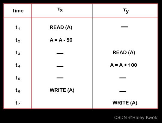

2. Dirty Read/ Temporary Update Problems (W-R Conflict)
The dirty read problem occurs when one transaction updates an item of the database, and somehow the transaction fails, and before the data gets rollback, the updated database item is accessed by another transaction. There comes the Read-Write Conflict between both transactions.

Then at time t4, transaction TY reads account A that will be read as $350.
Then at time t5, transaction TX rollbacks due to server problem, and the value changes back to $300 (as initially).
But the value for account A remains $350 for transaction TY as committed, which is the dirty read and therefore known as the Dirty Read Problem.
Value in one transaction has been rolled back, while the others have not.
3. Unrepeatable Read Problem (W-R Conflict)
Also known as Inconsistent Retrievals Problem that occurs when in a transaction, two different values are read for the same database item.

Within the same transaction TX, it reads two different values of account A, i.e., $ 300 initially, and after updation made by transaction TY, it reads $400. It is an unrepeatable read and is therefore known as the Unrepeatable read problem.
The incorrect summary problem:

Concurrency Control Protocols
Ensure ACID of the database
1. Lock Based Concurrency Control Protocol
In this type of protocol, any transaction cannot read or write data until it acquires an appropriate lock on it. There are two types of lock:
1. Shared lock
It is also known as a Read-only lock. In a shared lock, the data item can only read by the transaction. It can be shared between the transactions because when the transaction holds a lock, then it can’t update the data on the data item.
2. Exclusive lock
In the exclusive lock, the data item can be both reads as well as written by the transaction. This lock is exclusive, and in this lock, multiple transactions do not modify the same data simultaneously.
There are four types of lock protocols available:
1. Simplistic lock protocol
It is the simplest way of locking the data while transaction. Simplistic lock-based protocols allow all the transactions to get the lock on the data before insert or delete or update on it. It will unlock the data item after completing the transaction.
2. Pre-claiming Lock Protocol
Pre-claiming Lock Protocols evaluate the transaction to list all the data items on which they need locks.
Before initiating an execution of the transaction, it requests DBMS for all the lock on all those data items.
If all the locks are granted then this protocol allows the transaction to begin. When the transaction is completed then it releases all the lock.
If all the locks are not granted then this protocol allows the transaction to rolls back and waits until all the locks are granted.
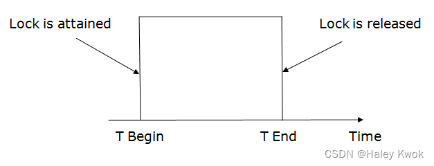
3. Two-phase locking (2PL)
The two-phase locking protocol divides the execution phase of the transaction into three parts.
- In the first part, when the execution of the transaction starts, it seeks permission for the lock it requires.
- In the second part, the transaction acquires all the locks.
- In the third phase, the transaction cannot demand any new locks. It only releases the acquired locks. The third phase is started as soon as the transaction releases its first lock.
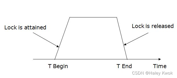
There are two phases of 2PL:
Growing phase: In the growing phase, a new lock on the data item may be acquired by the transaction, but none can be released.
Shrinking phase: In the shrinking phase, existing lock held by the transaction may be released, but no new locks can be acquired.
[Example]
Upgrading of lock (from S(a) to X (a)) is allowed in growing phase.
Downgrading of lock (from X(a) to S(a)) must be done in shrinking phase.

The following way shows how unlocking and locking work with 2-PL.
Transaction T1:
Growing phase: from step 1-3
Shrinking phase: from step 5-7
Lock point: at 3
Transaction T2:
Growing phase: from step 2-6
Shrinking phase: from step 8-9
Lock point: at 6
4. Strict Two-phase locking (Strict-2PL)
The first phase of Strict-2PL is similar to 2PL. In the first phase, after acquiring all the locks, the transaction continues to execute normally.
The only difference between 2PL and strict 2PL is that Strict-2PL does not release a lock after using it.
Strict-2PL waits until the whole transaction to commit, and then it releases all the locks at a time.
Strict-2PL protocol does not have shrinking phase of lock release.
It does not have cascading abort as 2PL does.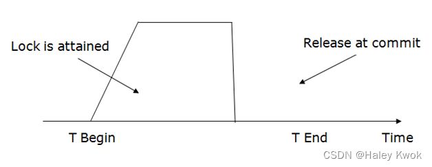
2. Time Stamp Concurrency Control Protocol
The Timestamp Ordering Protocol is used to order the transactions based on their Timestamps. The order of transaction is nothing but the ascending order of the transaction creation.
Basic Timestamp ordering protocol works as follows:
- Check the following condition whenever a transaction Ti issues a Read (X) operation:
If W_TS(X) >TS(Ti) then the operation is rejected.
If W_TS(X) <= TS(Ti) then the operation is executed.
Timestamps of all the data items are updated.
- Check the following condition whenever a transaction Ti issues a Write(X) operation:
If TS(Ti) < R_TS(X) then the operation is rejected.
If TS(Ti) < W_TS(X) then the operation is rejected and Ti is rolled back otherwise the operation is executed.
Where,
TS(TI) denotes the timestamp of the transaction Ti.
R_TS(X) denotes the Read time-stamp of data-item X.
W_TS(X) denotes the Write time-stamp of data-item X.
Advantages and Disadvantages of TO protocol:
TO protocol ensures serializability since the precedence graph is as follows:
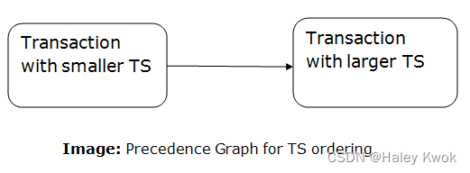
TS protocol ensures freedom from deadlock that means no transaction ever waits.
But the schedule may not be recoverable and may not even be cascade- free.
3. Validation Based Concurrency Control Protocol
Validation phase is also known as optimistic concurrency control technique. In the validation based protocol, the transaction is executed in the following three phases:
- Read phase: In this phase, the transaction T is read and executed. It is used to read the value of various data items and stores them in temporary local variables. It can perform all the write operations on temporary variables without an update to the actual database.
- Validation phase: In this phase, the temporary variable value will be validated against the actual data to see if it violates the serializability.
- Write phase: If the validation of the transaction is validated, then the temporary results are written to the database or system otherwise the transaction is rolled back.
Here each phase has the following different timestamps:
Start(Ti): It contains the time when Ti started its execution.
Validation (Ti): It contains the time when Ti finishes its read phase and starts its validation phase.
Finish(Ti): It contains the time when Ti finishes its write phase.
This protocol is used to determine the time stamp for the transaction for serialization using the time stamp of the validation phase, as it is the actual phase which determines if the transaction will commit or rollback.
Hence TS(T) = validation(T).
The serializability is determined during the validation process. It can’t be decided in advance.
While executing the transaction, it ensures a greater degree of concurrency and also less number of conflicts. Thus it contains transactions which have less number of rollbacks.
Multiple Granularity
Granularity: It is the size of data item allowed to lock.
It can be defined as hierarchically breaking up the database into blocks which can be locked.
The Multiple Granularity protocol enhances concurrency and reduces lock overhead.
It maintains the track of what to lock and how to lock.
It makes easy to decide either to lock a data item or to unlock a data item. This type of hierarchy can be graphically represented as a tree.
[Example]
Consider a tree which has four levels of nodes.
- The first level or higher level shows the entire database.
- The second level represents a node of type area. The higher level database consists of exactly these areas.
- The area consists of children nodes which are known as files. No file can be present in more than one area.
- Finally, each file contains child nodes known as records. The file has exactly those records that are its child nodes. No records represent in more than one file.
Hence, the levels of the tree starting from the top level are as follows:
- Database
- Area
- File
- Record
[Example]
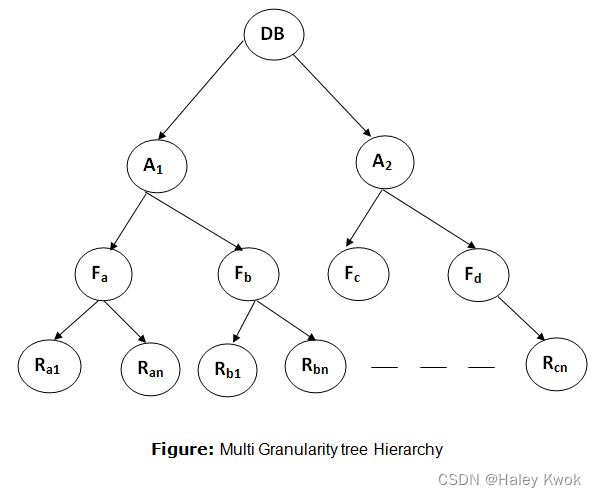
The highest level shows the entire database. The levels below are file, record, and fields. There are three additional lock modes with multiple granularity:
Intention Mode Lock
Intention-shared (IS): It contains explicit locking at a lower level of the tree but only with shared locks.
Intention-Exclusive (IX): It contains explicit locking at a lower level with exclusive or shared locks.
Shared & Intention-Exclusive (SIX): In this lock, the node is locked in shared mode, and some node is locked in exclusive mode by the same transaction.
Compatibility Matrix with Intention Lock Modes: The below table describes the compatibility matrix for these lock modes:

It uses the intention lock modes to ensure serializability. It requires that if a transaction attempts to lock a node, then that node must follow these protocols:
Transaction T1 should follow the lock-compatibility matrix.
Transaction T1 firstly locks the root of the tree. It can lock it in any mode.
If T1 currently has the parent of the node locked in either IX or IS mode, then the transaction T1 will lock a node in S or IS mode only.
If T1 currently has the parent of the node locked in either IX or SIX modes, then the transaction T1 will lock a node in X, SIX, or IX mode only.
If T1 has not previously unlocked any node only, then the Transaction T1 can lock a node.
If T1 currently has none of the children of the node-locked only, then Transaction T1 will unlock a node.
Observe that in multiple-granularity, the locks are acquired in top-down order, and locks must be released in bottom-up order.
If transaction T1 reads record Ra9 in file Fa, then transaction T1 needs to lock the database, area A1 and file Fa in IX mode. Finally, it needs to lock Ra2 in S mode.
If transaction T2 modifies record Ra9 in file Fa, then it can do so after locking the database, area A1 and file Fa in IX mode. Finally, it needs to lock the Ra9 in X mode.
If transaction T3 reads all the records in file Fa, then transaction T3 needs to lock the database, and area A in IS mode. At last, it needs to lock Fa in S mode.
If transaction T4 reads the entire database, then T4 needs to lock the database in S mode.
Recovery with Concurrent Transaction
Whenever more than one transaction is being executed, then the interleaved of logs occur. During recovery, it would become difficult for the recovery system to backtrack all logs and then start recovering.
To ease this situation, ‘checkpoint’ concept is used by most DBMS.
Refer to Transaction Processing Concept
When the system recovers from crash, it will construct an undo-list and a redo-list. The log records for transactions on the undo list must be processed in reverse order, while those log records for transactions on the redo-list must be processed in a sequential order.
In the undo phase, the system will roll back all transactions in the undo-list by scanning the log backward from the end. When it finds a log record belonging to a transaction in the undo list, it performs the undo operation as if the log record was found during the rollback of a failed transaction found during the rollback of a failed transaction. Normal transaction processing can be resumed after the undo phase of recovery is over.
In the redo phase, the system replays updates of all transactions by scanning the log forward from the last checkpoint. Some transactions in the redo log must continue in the same order in which the operations are written in the log. Redo operations must be idempotent and executing them again and again is equivalent to executing them only once and the entire recovery process should be idempotent.
Chapter 9: DDT
Lab 1 Table Definition, Manipulation and Simple Queries
Link to SQL
ssh [email protected]

# enter your password (the one that you use to log in to department’s PC)

apollo apollo2

source /compsoft/app/oracle/dbms.bashrc

sqlplus


# Your Oracle account is opened as follows
Username: "20060241d"@dbms
Password: iyrhpast

exit
Import .SQL
假如文件名称有空格 应该输入/反斜杠, 比如/Users/haleyk/Desktop/COMP2411\Database\Systems/Lab/LabData.sql
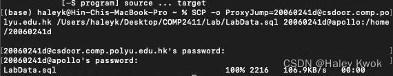
scp -o ProxyJump=[email protected] LabData.sql /Users/haleyk/Desktop/COMP2411/Lab/LabData.sql 20060241d@apollo:/home/20060241d

# load the data after entering the SQL*PLUS
SQL*PLUS:20060241d>@LabData.sql
Exercise
After each insert, update and delete operations that would modify the data in the database, you are suggested to do a “COMMIT” operation to ensure the changes take effect immediately
1.1 Common Data Types
CHAR (n) n = maximum length of char string
NUMBER (n,d) n = maximum
e.g., 1234.56:number(6,2)
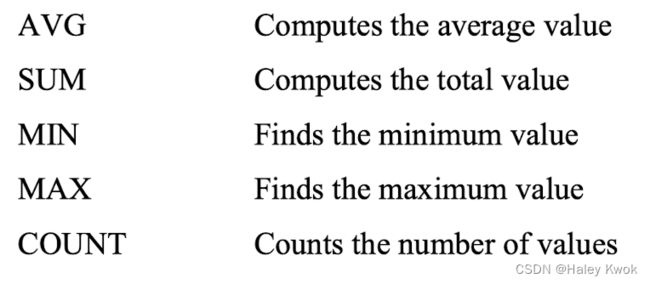
of digits d = maximum number of digits right of decimal
DATE The relevant data plus the actual time of day
LONG Up to 65,536 characters (64K) may be stored per field
RAW Raw binary data
1.2 NULL values
To forbid NULL values in a column, enter the NOT NULL clause at the end of the column information
2.1 Inserting Tuples into Tables
User variables & (or called substitution variable) can be used to help reduce the tedium of data insertion. For example, to insert rows into the DEPT table, enter the following command:

2.2 Altering Tables
You may add a new column or change the length of an existing column by using the ALTER TABLE command with either the ADD or MODIFY parameters. Note that you may not reduce the width of a column if it contains data, nor may you change data type unless the column is empty.
Change the length of column LOC in table DEPT from 15 to 20
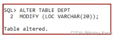
3.1 Select
SELECT some columns
FROM some tables
WHERE certain conditions are met
AND/OR
Lab 2 Queries, Arithmetic Expressions and Functions
1.1 Selecting Rows within a Certain Range
BETWEEN/ NOT BETWEEN
1.2 Selecting Rows That Match a Value in List
SQL > SELECT ENAME, JOB, DEPTNO
FROM EMP
WHERE JOB IN (‘CLERK’, ‘ANALYST’, ‘SALESMAN’);
/NOT IN
1.3 Selecting Rows That Match a Character Pattern
% The percent character represents any string of zero or more characters
Start begins with M/ end with N
SQL > SELECT ENAME, JOB, DEPTNO
FROM EMP
WHERE ENAME LIKE ‘M%‘;
/’%N’
_ The underscore character means a single character position
2.1 Ordering Rows
Ascending order:
SELECT SAL, JOB, ENAME
FROM EMP
WHERE DEPTNO = 30
ORDER BY SAL;
Descending order:
SELECT SAL, JOB, ENAME,
FROM EMP
WHERE DEPTNO = 30
ORDER BY SAL DESC;
2.2 Ordering Rows Using Multiple Columns
CLERKs are in descending salary order, and all the MANAGERs are in descending salary order, etc.
SELECT JOB, SAL, ENAME
FROM EMP
ORDER BY JOB, SAL DESC;
2.3 Ordering Rows By Columns With NULL Values
SELECT … ORDER BY … ASC/DESC NULLS FIRST/LAST;
3.1 Arithmetic Expressions

SELECT ENAME, SAL, COMM, SAL+COMM
FROM EMP
WHERE JOB = ‘SALESMAN’;
SELECT ENAME, SAL, COMM
FROM EMP
WHERE COMM > 0.25 * SAL;
More than one arithmetic expressions can be used:
SELECT ENAME, SAL, COMM, (SAL+COMM)*12
FROM EMP
WHERE JOB = ‘SALESMAN’;
3.2 Arithmetic Expressions with ORDER BY
SELECT ENAME, COMM/SAL, COMM, SAL
FROM EMP
WHERE JOB = ‘SALESMAN’
ORDER BY COMM/SAL DESC;
3.3 The NULL Function
The expression SAL+NVL(COMM, 0) will return a value equal to SAL + 0 when the COMM field is null.
SELECT ENAME, JOB, SAL, COMM, SAL+NVL(COMM, 0)
FROM EMP
WHERE DEPTNO = 30;
3.4 Column Labels
Use _ or “” to avoid any blanks
SELECT ENAME, JOB, SAL SALARY, COMM COMMISSION,
SAL+NVL(COMM, 0) TOTAL_COMPENSATION
FROM EMP
WHERE DEPTNO = 30;
“TOTAL COMPENSATION”
4.1 Arithmetic Functions (ROUND)
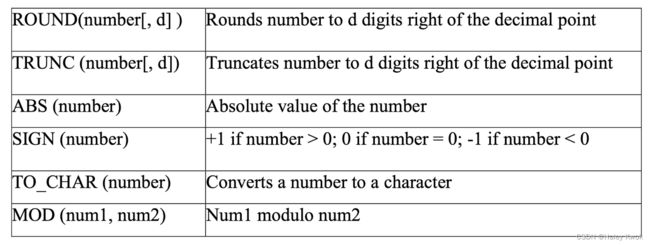
Select the results in three separate columns: unrounded, rounded to the nearest dollar, and rounded to the nearest cent.
SELECT ENAME, SAL, SAL/22, ROUND(SAL/22, 0), ROUND(SAL/22, 2)
FROM EMP
WHERE DEPTNO = 30;
SELECT ENAME, SAL MONTHLY, ROUND(SAL/22,2) DAILY,ROUND(SAL/(22*8),2) HOURLY
FROM EMP
WHERE DEPTNO = 30;
TRUNC(SAL/22,2) DAILY 截断
5.1 Character String Functions

Concatenate the DNAME column to the LOC column separated by a blank space, a dash and another blank space (‘ – ‘)
SELECT DNAME || ‘ – ‘ || LOC DEPARTMENTS
FROM DEPT;
Abbreviate the department name to the first 5 characters of the department name.
SELECT SUBSTR(DNAME,1,5)
FROM DEPT
SELECT ENAME, UPPER(ENAME), LOWER(ENAME)
FROM EMP
WHERE UPPER(ENAME) = UPPER(‘Ward’);
SELECT DNAME, LENGTH(DNAME)
FROM DEPT;
Lab 3 Aggregate Functions, ‘Group By’ and ‘Having’ Clauses
In all the examples so far, we have selected values stored in each row of a table (like SAL), or values calculated for each row (like SAL*12).
1.1 Selecting Summary Information from One Group
Find the average salary for clerk
SELECT AVG(SAL)
FROM EMP
WHERE JOB = 'CLERK';
Find the total salary and total commission for salesmen
SELECT SUM(SAL), SUM(COMM)
FROM EMP
WHERE JOB = ‘SALESMAN’;
Find the highest and lowest paid employee salaries and the difference between them.
SELECT MAX(SAL), MIN(SAL), MAX(SAL) – MIN(SAL)
FROM EMP;
2.1 Sub-query
In standard SQL, you may NOT have both aggregates and non-aggregates in the same SELECT list. For example, SELECT ENAME, AVG(SAL) is an error. This is because ENAME is an attribute of each row selected and AVG(SAL) is an attribute of all the rows selected. So if you want to find the name and salary of the employee (or employees) who receive the maximum salary, you cannot use the above query
Find the name and salary of the employee (or employees) who receive the maximum salary.
SELECT ENAME, JOB, SAL
FROM EMP
WHERE SAL =
(SELECT MAX(SAL) FROM EMP);
2.2 DISTINCT
Count the number of different jobs held by employees in department 30
SELECT COUNT(DISTINCT JOB)
FROM EMP
WHERE DEPTNO = 30
3.1 SELECTING SUMMARY INFORMATION FROM GROUPS – GROUP BY
List the department number and average salary of each department
female or male -> cannot be ordered by
SELECT DEPTNO, AVG(SAL)
FROM EMP
GROUP BY DEPTNO;
Find each department’s average annual salary for all its employees except the managers and the president
SELECT DEPTNO, AVG(SAL)*12
FROM EMP
WHERE JOB NOT IN (‘MANAGER’, ‘PRESIDENT’)
GROUP BY DEPTNO;
Issue the same query as above except list the department name rather than the department number
SELECT DNAME, JOB, COUNT(*), AVG(SAL)*12
FROM EMP, DEPT
WHERE DEPT.DEPTNO = EMP.DEPTNO
GROUP BY DNAME, JOB
EMP, DEPT got the same DEPTNO THUS, DEPT.DEPTNO, EMP.DEPTNO are used to diverse them However, for SALARY.T SALARY.S, it is the same table, but used for more than one times.
3.2 SPECIFYING A SEARCH-CONDITION FOR GROUPS – HAVING
Search-conditions for individual rows are specified in the WHERE clause, for groups, you should use HAVING clause to do specification.
List the average annual salary for all job groups having more than 2 employees in
the group.
SELECT JOB, COUNT(*), AVG(SAL)*12
FROM EMP
GROUP BY JOB
HAVING COUNT(*) > 2;
3.3 More on Sub-query
List the job groups that have an average salary greater than the average salary of managers.
SELECT JOB, AVG(SAL)
FROM EMP
GROUP BY JOB
HAVING AVG(SAL) >
(SELECT AVG(SAL) FROM EMP
WHERE JOB = ‘MANAGER’);
4.1 4 EFFECTS OF NULL VALUES ON GROUP FUNCTIONS
Null values do not participate in the computation of group functions.
SELECT SUM(SAL), COUNT(SAL), AVG(SAL), SUM(COMM),
COUNT (COMM), AVG(COMM)
FROM EMP
WHERE DEPTNO = 30;
List the average commission of employees who receive a commission, and the average commission of all employees (treating employees who do not receive a commission as receiving a zero commission).
SELECT AVG(COMM), AVG(NVL(COMM, 0))
FROM EMP
WHERE DEPTNO = 30;
5 FORMATING QUERY RESULTS INTO A REPORT
In this section, you will learn some more SQL*Plus commands to improve the appearance (format) of a query result. The commands to be covered in this section