MachineLearning 5. 癌症诊断和分子分型方法之支持向量机(SVM)

点击关注,桓峰基因
桓峰基因
生物信息分析,SCI文章撰写及生物信息基础知识学习:R语言学习,perl基础编程,linux系统命令,Python遇见更好的你
92篇原创内容
公众号
桓峰基因的教程不但教您怎么使用,还会定期分析一些相关的文章,学会教程只是基础,但是如果把分析结果整合到文章里面才是目的,觉得我们这些教程还不错,并且您按照我们的教程分析出来不错的结果发了文章记得告知我们,并在文章中感谢一下我们哦!
公司英文名称:Kyoho Gene Technology (Beijing) Co.,Ltd.
如果您觉得这些确实没基础,需要专业的生信人员帮助分析,直接扫码加微信,我们24小时在线!!微信号:nihaooo123

****支持向量机(SVM)在癌症诊断和分子分型中表现强健,一般文章都使用Lasso回归等进行预后分析,当作到机器学习分子分型等可能文章就上了更高的一个台阶,这就是为什么现在AI精准医疗为什么这么火热,人工智能完全可以降低误诊和滥用药物的可能,抽管血就能准确的知道得了什么病,需要使用哪种药,还是蛮NB的!
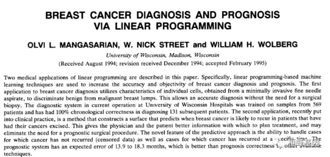
前言
支持向量机(SVM)方法是一种数据驱动的分类任务求解方法。研究表明,与基于其他方法(如人工神经网络)的分类器相比,该方法产生更低的预测误差,特别是在考虑样本描述的大量特征时。本文概述了支持向量机方法的原理和主要原理,并介绍了支持向量机方法在传统生物信息学研究领域的成功应用。本文综述了支持向量机相关技术的最新进展,这些进展可能会对未来的功能基因组学和化学基因组学项目产生影响。
基本原理
支持向量机(Support Vector Machine, SVM)是一类按监督学习(supervised learning)方式对数据进行二元分类的广义线性分类器(generalized linear classifier),其决策边界是对学习样本求解的最大边距超平面(maximum-margin hyperplane)。
支持向量机还代表了一种强大的技术,用于一般(非线性)分类、回归和异常点检测的监督学习方法,具有直观的模型表示。SVM使用铰链损失函数(hinge loss)计算经验风险(empirical risk)并在求解系统中加入了正则化项以优化结构风险(structural risk),是一个具有稀疏性和稳健性的分类器。SVM可以通过核方法(kernel method)进行非线性分类,是常见的核学习(kernel learning)方法之一。支持向量机的优点是:在高维空间有效。在维数大于样本数的情况下仍然有效。在决策函数中使用训练点的子集(称为支持向量),因此它也是有效的内存。通用性:可以指定不同的核函数作为决策函数。提供了通用内核,但也可以指定自定义内核。支持向量机的缺点包括:如果特征的数量远远大于样本的数量,在选择核函数时避免过拟合,正则项是至关重要的。支持向量机不直接提供概率估计,这些估计是使用昂贵的五次交叉验证计算出来的。
实例解析
1. 软件安装
这里我们主要使用e1071和class两个软件包,其他都为数据处理过程中需要使用软件包,如下:
if (!require(class)) install.packages("class")
if (!require(e1071)) install.packages("e1071")
if (!require(caret)) install.packages("caret")

library(class)
library(e1071)
library(caret)
library(reshape2)
library(ggplot2)
2. 数据读取
数据来源《机器学习与R语言》书中,具体来自UCI机器学习仓库。地址:http://archive.ics.uci.edu/ml/machine-learning-databases/breast-cancer-wisconsin/ 下载wbdc.data和wbdc.names这两个数据集,数据经过整理,成为面板数据。查看数据结构,其中第一列为id列,无特征意义,需要删除。第二列diagnosis为响应变量,字符型,一般在R语言中分类任务都要求响应变量为因子类型,因此需要做数据类型转换。剩余的为预测变量,数值类型。查看数据维度,568个样本,32个特征(包括响应特征)。
BreastCancer <- read.csv("wisc_bc_data.csv", stringsAsFactors = FALSE)
str(BreastCancer)
## 'data.frame':	568 obs. of  32 variables:
##  $ id                     : int  842517 84300903 84348301 84358402 843786 844359 84458202 844981 84501001 845636 ...
##  $ diagnosis              : chr  "M" "M" "M" "M" ...
##  $ radius_mean            : num  20.6 19.7 11.4 20.3 12.4 ...
##  $ texture_mean           : num  17.8 21.2 20.4 14.3 15.7 ...
##  $ perimeter_mean         : num  132.9 130 77.6 135.1 82.6 ...
##  $ area_mean              : num  1326 1203 386 1297 477 ...
##  $ smoothness_mean        : num  0.0847 0.1096 0.1425 0.1003 0.1278 ...
##  $ compactne_mean         : num  0.0786 0.1599 0.2839 0.1328 0.17 ...
##  $ concavity_mean         : num  0.0869 0.1974 0.2414 0.198 0.1578 ...
##  $ concave_points_mean    : num  0.0702 0.1279 0.1052 0.1043 0.0809 ...
##  $ symmetry_mean          : num  0.181 0.207 0.26 0.181 0.209 ...
##  $ fractal_dimension_mean : num  0.0567 0.06 0.0974 0.0588 0.0761 ...
##  $ radius_se              : num  0.543 0.746 0.496 0.757 0.335 ...
##  $ texture_se             : num  0.734 0.787 1.156 0.781 0.89 ...
##  $ perimeter_se           : num  3.4 4.58 3.44 5.44 2.22 ...
##  $ area_se                : num  74.1 94 27.2 94.4 27.2 ...
##  $ smoothness_se          : num  0.00522 0.00615 0.00911 0.01149 0.00751 ...
##  $ compactne_se           : num  0.0131 0.0401 0.0746 0.0246 0.0335 ...
##  $ concavity_se           : num  0.0186 0.0383 0.0566 0.0569 0.0367 ...
##  $ concave_points_se      : num  0.0134 0.0206 0.0187 0.0188 0.0114 ...
##  $ symmetry_se            : num  0.0139 0.0225 0.0596 0.0176 0.0216 ...
##  $ fractal_dimension_se   : num  0.00353 0.00457 0.00921 0.00511 0.00508 ...
##  $ radius_worst           : num  25 23.6 14.9 22.5 15.5 ...
##  $ texture_worst          : num  23.4 25.5 26.5 16.7 23.8 ...
##  $ perimeter_worst        : num  158.8 152.5 98.9 152.2 103.4 ...
##  $ area_worst             : num  1956 1709 568 1575 742 ...
##  $ smoothness_worst       : num  0.124 0.144 0.21 0.137 0.179 ...
##  $ compactne_worst        : num  0.187 0.424 0.866 0.205 0.525 ...
##  $ concavity_worst        : num  0.242 0.45 0.687 0.4 0.535 ...
##  $ concave_points_worst   : num  0.186 0.243 0.258 0.163 0.174 ...
##  $ symmetry_worst         : num  0.275 0.361 0.664 0.236 0.399 ...
##  $ fractal_dimension_worst: num  0.089 0.0876 0.173 0.0768 0.1244 ...
BreastCancer[1:5, 1:5]
##         id diagnosis radius_mean texture_mean perimeter_mean
## 1   842517         M       20.57        17.77         132.90
## 2 84300903         M       19.69        21.25         130.00
## 3 84348301         M       11.42        20.38          77.58
## 4 84358402         M       20.29        14.34         135.10
## 5   843786         M       12.45        15.70          82.57
dim(BreastCancer)
## [1] 568  32
table(BreastCancer$diagnosis)
##
##   B   M
## 357 211
sum(is.na(data))  # 检测数据是否有缺失
## [1] 0
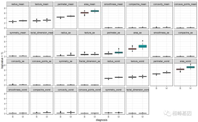
数据分布比较恶性和良性之间的差距,如下:
bc <- BreastCancer[, -1]
bc.melt <- melt(bc, id.var = "diagnosis")
head(bc.melt)
##   diagnosis    variable value
## 1         M radius_mean 20.57
## 2         M radius_mean 19.69
## 3         M radius_mean 11.42
## 4         M radius_mean 20.29
## 5         M radius_mean 12.45
## 6         M radius_mean 18.25
ggplot(data = bc.melt, aes(x = diagnosis, y = log(value + 1), fill = diagnosis)) +
    geom_boxplot() + theme_bw() + facet_wrap(~variable, ncol = 8)
数据变量之间的相关性,如下:
library(tidyverse)
data <- select(BreastCancer, -1) %>%
    mutate_at("diagnosis", as.factor)
corrplot::corrplot(cor(data[, -1]))

数据分割将原始数据分割成训练数据和测试数据,测试数据不参与训练建模,将根据模型在测试数据中的表现来选择最优模型参数。
一般做数据分割会留70%的训练数据和30%的测试数据,当然这个比例可以更改,但是一般是训练数据要大于测试数据,用来保证模型学习的充分性。
此外,在做分类任务时,有一个需要额外考虑的问题就是需要尽可能保证训练数据和测试数据中正负样本的比例相近。这里采用「分层抽样」来完成这个任务。
library(sampling)
set.seed(123)
# 每层抽取70%的数据
train_id <- strata(data, "diagnosis", size = rev(round(table(data$diagnosis) * 0.7)))$ID_unit
# 训练数据
train_data <- data[train_id, ]
# 测试数据
test_data <- data[-train_id, ]

# 查看训练、测试数据中正负样本比例
prop.table(table(train_data$diagnosis))
##
##         B         M
## 0.6281407 0.3718593

prop.table(table(test_data$diagnosis))
##
##         B         M
## 0.6294118 0.3705882
3. 实例操作
一个简单的向后选择,也就是递归特征消除(RFE)算法。这里面涉及到四种核函数的计算方法,我们每种方法都做一遍,最后汇总比较哪种方法的准确性最高,敏感度更好!

1. linear
set.seed(123)
linear.tune <- tune.svm(diagnosis ~ ., data = train_data, kernel = "linear", cost = c(0.001,
    0.01, 0.1, 1, 5, 10))
summary(linear.tune)
##
## Parameter tuning of 'svm':
##
## - sampling method: 10-fold cross validation
##
## - best parameters:
##  cost
##   0.1
##
## - best performance: 0.03012821
##
## - Detailed performance results:
##    cost      error dispersion
## 1 1e-03 0.05782051 0.05163412
## 2 1e-02 0.04019231 0.03397375
## 3 1e-01 0.03012821 0.03504404
## 4 1e+00 0.03012821 0.03082705
## 5 5e+00 0.03519231 0.02964077
## 6 1e+01 0.04512821 0.03293816
best.linear <- linear.tune$best.model
tune.test <- predict(best.linear, newdata = test_data)
table(tune.test, test_data$diagnosis)
##
## tune.test   B   M
##         B 106   3
##         M   1  60
confusionMatrix(tune.test, test_data$diagnosis, positive = "B")
## Confusion Matrix and Statistics
##
##           Reference
## Prediction   B   M
##          B 106   3
##          M   1  60
##
##                Accuracy : 0.9765
##                  95% CI : (0.9409, 0.9936)
##     No Information Rate : 0.6294
##     P-Value [Acc > NIR] : <2e-16
##
##                   Kappa : 0.9492
##
##  Mcnemar's Test P-Value : 0.6171
##
##             Sensitivity : 0.9907
##             Specificity : 0.9524
##          Pos Pred Value : 0.9725
##          Neg Pred Value : 0.9836
##              Prevalence : 0.6294
##          Detection Rate : 0.6235
##    Detection Prevalence : 0.6412
##       Balanced Accuracy : 0.9715
##
##        'Positive' Class : B
##
# Accuracy : 0.9765 svmLinear
set.seed(123)
rfeCNTL <- rfeControl(functions = lrFuncs, method = "cv", number = 10)
svmLinear <- rfe(train_data[, -1], train_data[, 1], sizes = c(7, 6, 5, 4), rfeControl = rfeCNTL,
    method = "svmLinear")
svmLinear
##
## Recursive feature selection
##
## Outer resampling method: Cross-Validated (10 fold)
##
## Resampling performance over subset size:
##
##  Variables Accuracy  Kappa AccuracySD KappaSD Selected
##          4   0.8941 0.7653    0.07515 0.17331
##          5   0.9068 0.7983    0.05515 0.12066
##          6   0.9244 0.8375    0.05201 0.11170
##          7   0.9471 0.8852    0.03660 0.07977        *
##         30   0.9396 0.8721    0.04036 0.08635
##
## The top 5 variables (out of 7):
##    fractal_dimension_se, fractal_dimension_worst, smoothness_mean, concave_points_mean, texture_mean
vec <- names(coefficients(svmLinear$fit))[-1]
var <- paste(vec, collapse = "+")
fun <- as.formula(paste("diagnosis", "~", var))
svm <- svm(fun, data = train_data, kernel = "linear")
Linear.predict = predict(svm, newdata = test_data[, vec])
table(Linear.predict, test_data$diagnosis)
##
## Linear.predict   B   M
##              B 105   8
##              M   2  55
confusionMatrix(Linear.predict, test_data$diagnosis, positive = "B")
## Confusion Matrix and Statistics
##
##           Reference
## Prediction   B   M
##          B 105   8
##          M   2  55
##
##                Accuracy : 0.9412
##                  95% CI : (0.8945, 0.9714)
##     No Information Rate : 0.6294
##     P-Value [Acc > NIR] : <2e-16
##
##                   Kappa : 0.8714
##
##  Mcnemar's Test P-Value : 0.1138
##
##             Sensitivity : 0.9813
##             Specificity : 0.8730
##          Pos Pred Value : 0.9292
##          Neg Pred Value : 0.9649
##              Prevalence : 0.6294
##          Detection Rate : 0.6176
##    Detection Prevalence : 0.6647
##       Balanced Accuracy : 0.9272
##
##        'Positive' Class : B
##
# Accuracy : 0.9412
2. poly
################## tune the poly only
set.seed(123)
poly.tune <- tune.svm(diagnosis ~ ., data = train_data, kernel = "polynomial", degree = c(3,
    4, 5), coef0 = c(0.1, 0.5, 1, 2, 3, 4))
summary(poly.tune)
##
## Parameter tuning of 'svm':
##
## - sampling method: 10-fold cross validation
##
## - best parameters:
##  degree coef0
##       3     1
##
## - best performance: 0.02769231
##
## - Detailed performance results:
##    degree coef0      error dispersion
## 1       3   0.1 0.07038462 0.04063291
## 2       4   0.1 0.11557692 0.05439623
## 3       5   0.1 0.14583333 0.05660357
## 4       3   0.5 0.04269231 0.04274060
## 5       4   0.5 0.04019231 0.03784169
## 6       5   0.5 0.04269231 0.03755119
## 7       3   1.0 0.02769231 0.04183104
## 8       4   1.0 0.03269231 0.04113567
## 9       5   1.0 0.03769231 0.03794742
## 10      3   2.0 0.03019231 0.03523951
## 11      4   2.0 0.03769231 0.04144616
## 12      5   2.0 0.04269231 0.03151865
## 13      3   3.0 0.03019231 0.03321045
## 14      4   3.0 0.03762821 0.03390515
## 15      5   3.0 0.04262821 0.03132839
## 16      3   4.0 0.03519231 0.03598947
## 17      4   4.0 0.04512821 0.03691477
## 18      5   4.0 0.04012821 0.03379204
best.poly <- poly.tune$best.model
poly.test <- predict(best.poly, newdata = test_data)
table(poly.test, test_data$diagnosis)
##
## poly.test   B   M
##         B 107   2
##         M   0  61
confusionMatrix(poly.test, test_data$diagnosis, positive = "B")
## Confusion Matrix and Statistics
##
##           Reference
## Prediction   B   M
##          B 107   2
##          M   0  61
##
##                Accuracy : 0.9882
##                  95% CI : (0.9581, 0.9986)
##     No Information Rate : 0.6294
##     P-Value [Acc > NIR] : <2e-16
##
##                   Kappa : 0.9746
##
##  Mcnemar's Test P-Value : 0.4795
##
##             Sensitivity : 1.0000
##             Specificity : 0.9683
##          Pos Pred Value : 0.9817
##          Neg Pred Value : 1.0000
##              Prevalence : 0.6294
##          Detection Rate : 0.6294
##    Detection Prevalence : 0.6412
##       Balanced Accuracy : 0.9841
##
##        'Positive' Class : B
##
# Accuracy : 0.9882 svmPoly
set.seed(123)
svmPoly <- rfe(train_data[, -1], train_data[, 1], sizes = c(7, 6, 5, 4), rfeControl = rfeCNTL,
    method = "svmPoly")
svmPoly
##
## Recursive feature selection
##
## Outer resampling method: Cross-Validated (10 fold)
##
## Resampling performance over subset size:
##
##  Variables Accuracy  Kappa AccuracySD KappaSD Selected
##          4   0.8941 0.7653    0.07515 0.17331
##          5   0.9068 0.7983    0.05515 0.12066
##          6   0.9244 0.8375    0.05201 0.11170
##          7   0.9471 0.8852    0.03660 0.07977        *
##         30   0.9396 0.8721    0.04036 0.08635
##
## The top 5 variables (out of 7):
##    fractal_dimension_se, fractal_dimension_worst, smoothness_mean, concave_points_mean, texture_mean
vec <- names(coefficients(svmPoly$fit))[-1]
var <- paste(vec, collapse = "+")
fun <- as.formula(paste("diagnosis", "~", var))
svm <- svm(fun, data = train_data, kernel = "poly")
Poly.predict = predict(svm, newdata = test_data[, vec])
table(Poly.predict, test_data$diagnosis)
##
## Poly.predict   B   M
##            B 105  24
##            M   2  39
confusionMatrix(Poly.predict, test_data$diagnosis, positive = "B")
## Confusion Matrix and Statistics
##
##           Reference
## Prediction   B   M
##          B 105  24
##          M   2  39
##
##                Accuracy : 0.8471
##                  95% CI : (0.784, 0.8976)
##     No Information Rate : 0.6294
##     P-Value [Acc > NIR] : 3.183e-10
##
##                   Kappa : 0.6468
##
##  Mcnemar's Test P-Value : 3.814e-05
##
##             Sensitivity : 0.9813
##             Specificity : 0.6190
##          Pos Pred Value : 0.8140
##          Neg Pred Value : 0.9512
##              Prevalence : 0.6294
##          Detection Rate : 0.6176
##    Detection Prevalence : 0.7588
##       Balanced Accuracy : 0.8002
##
##        'Positive' Class : B
##
# Accuracy : 0.8471
3. radial
########################## tune the radial
set.seed(123)
rbf.tune <- tune.svm(diagnosis ~ ., data = train_data, kernel = "radial", gamma = c(0.1,
    0.5, 1, 2, 3, 4))
summary(rbf.tune)
##
## Parameter tuning of 'svm':
##
## - sampling method: 10-fold cross validation
##
## - best parameters:
##  gamma
##    0.1
##
## - best performance: 0.05012821
##
## - Detailed performance results:
##   gamma      error dispersion
## 1   0.1 0.05012821 0.05773645
## 2   0.5 0.22833333 0.10924627
## 3   1.0 0.37185897 0.07966989
## 4   2.0 0.37185897 0.07966989
## 5   3.0 0.37185897 0.07966989
## 6   4.0 0.37185897 0.07966989
best.rbf <- rbf.tune$best.model
rbf.test <- predict(best.rbf, newdata = test_data)
table(rbf.test, test_data$diagnosis)
##
## rbf.test   B   M
##        B 104   3
##        M   3  60
confusionMatrix(rbf.test, test_data$diagnosis, positive = "B")
## Confusion Matrix and Statistics
##
##           Reference
## Prediction   B   M
##          B 104   3
##          M   3  60
##
##                Accuracy : 0.9647
##                  95% CI : (0.9248, 0.9869)
##     No Information Rate : 0.6294
##     P-Value [Acc > NIR] : <2e-16
##
##                   Kappa : 0.9243
##
##  Mcnemar's Test P-Value : 1
##
##             Sensitivity : 0.9720
##             Specificity : 0.9524
##          Pos Pred Value : 0.9720
##          Neg Pred Value : 0.9524
##              Prevalence : 0.6294
##          Detection Rate : 0.6118
##    Detection Prevalence : 0.6294
##       Balanced Accuracy : 0.9622
##
##        'Positive' Class : B
##
# Accuracy : 0.9647 svmRadial
set.seed(123)
svmRadial <- rfe(train_data[, -1], train_data[, 1], sizes = c(7, 6, 5, 4), rfeControl = rfeCNTL,
    method = "svmRadial")
svmRadial
##
## Recursive feature selection
##
## Outer resampling method: Cross-Validated (10 fold)
##
## Resampling performance over subset size:
##
##  Variables Accuracy  Kappa AccuracySD KappaSD Selected
##          4   0.8941 0.7653    0.07515 0.17331
##          5   0.9068 0.7983    0.05515 0.12066
##          6   0.9244 0.8375    0.05201 0.11170
##          7   0.9471 0.8852    0.03660 0.07977        *
##         30   0.9396 0.8721    0.04036 0.08635
##
## The top 5 variables (out of 7):
##    fractal_dimension_se, fractal_dimension_worst, smoothness_mean, concave_points_mean, texture_mean
vec <- names(coefficients(svmRadial$fit))[-1]
var <- paste(vec, collapse = "+")
fun <- as.formula(paste("diagnosis", "~", var))
svm <- svm(fun, data = train_data, kernel = "radial")
Radial.predict = predict(svm, newdata = test_data[, vec])
table(Radial.predict, test_data$diagnosis)
##
## Radial.predict   B   M
##              B 104  12
##              M   3  51
confusionMatrix(Radial.predict, test_data$diagnosis, positive = "B")
## Confusion Matrix and Statistics
##
##           Reference
## Prediction   B   M
##          B 104  12
##          M   3  51
##
##                Accuracy : 0.9118
##                  95% CI : (0.8586, 0.9498)
##     No Information Rate : 0.6294
##     P-Value [Acc > NIR] : < 2e-16
##
##                   Kappa : 0.8051
##
##  Mcnemar's Test P-Value : 0.03887
##
##             Sensitivity : 0.9720
##             Specificity : 0.8095
##          Pos Pred Value : 0.8966
##          Neg Pred Value : 0.9444
##              Prevalence : 0.6294
##          Detection Rate : 0.6118
##    Detection Prevalence : 0.6824
##       Balanced Accuracy : 0.8907
##
##        'Positive' Class : B
##
# Accuracy : 0.9118
4. sigmoid
################### tune the sigmoid
set.seed(123)
sigmoid.tune <- tune.svm(diagnosis ~ ., data = train_data, kernel = "sigmoid", gamma = c(0.1,
    0.5, 1, 2, 3, 4), coef0 = c(0.1, 0.5, 1, 2, 3, 4))
summary(sigmoid.tune)
##
## Parameter tuning of 'svm':
##
## - sampling method: 10-fold cross validation
##
## - best parameters:
##  gamma coef0
##    0.1   0.1
##
## - best performance: 0.06512821
##
## - Detailed performance results:
##    gamma coef0      error dispersion
## 1    0.1   0.1 0.06512821 0.04428204
## 2    0.5   0.1 0.10807692 0.04746880
## 3    1.0   0.1 0.11314103 0.04922072
## 4    2.0   0.1 0.09057692 0.06814132
## 5    3.0   0.1 0.10051282 0.04565635
## 6    4.0   0.1 0.10538462 0.05611503
## 7    0.1   0.5 0.11282051 0.06022382
## 8    0.5   0.5 0.12064103 0.05782179
## 9    1.0   0.5 0.12576923 0.04912932
## 10   2.0   0.5 0.10557692 0.05879917
## 11   3.0   0.5 0.10051282 0.04867745
## 12   4.0   0.5 0.11820513 0.04298665
## 13   0.1   1.0 0.11538462 0.04558048
## 14   0.5   1.0 0.13064103 0.03682139
## 15   1.0   1.0 0.14064103 0.03928394
## 16   2.0   1.0 0.09788462 0.04767979
## 17   3.0   1.0 0.09064103 0.06521765
## 18   4.0   1.0 0.11801282 0.06337151
## 19   0.1   2.0 0.14589744 0.05171576
## 20   0.5   2.0 0.14076923 0.05047278
## 21   1.0   2.0 0.14814103 0.05686768
## 22   2.0   2.0 0.08801282 0.03407708
## 23   3.0   2.0 0.10794872 0.05531440
## 24   4.0   2.0 0.09807692 0.06531545
## 25   0.1   3.0 0.18621795 0.06910882
## 26   0.5   3.0 0.16333333 0.05563423
## 27   1.0   3.0 0.14083333 0.04645070
## 28   2.0   3.0 0.11307692 0.05173871
## 29   3.0   3.0 0.09570513 0.07013109
## 30   4.0   3.0 0.11057692 0.05076956
## 31   0.1   4.0 0.26929487 0.08718601
## 32   0.5   4.0 0.17589744 0.06772675
## 33   1.0   4.0 0.14326923 0.06472296
## 34   2.0   4.0 0.14301282 0.05738479
## 35   3.0   4.0 0.11064103 0.05580090
## 36   4.0   4.0 0.09794872 0.05577439

best.sigmoid <- sigmoid.tune$best.model
sigmoid.test <- predict(best.sigmoid, newdata = test_data)
table(sigmoid.test, test_data$diagnosis)
##
## sigmoid.test   B   M
##            B 103  11
##            M   4  52
confusionMatrix(sigmoid.test, test_data$diagnosis, positive = "B")
## Confusion Matrix and Statistics
##
##           Reference
## Prediction   B   M
##          B 103  11
##          M   4  52
##
##                Accuracy : 0.9118
##                  95% CI : (0.8586, 0.9498)
##     No Information Rate : 0.6294
##     P-Value [Acc > NIR] : <2e-16
##
##                   Kappa : 0.8064
##
##  Mcnemar's Test P-Value : 0.1213
##
##             Sensitivity : 0.9626
##             Specificity : 0.8254
##          Pos Pred Value : 0.9035
##          Neg Pred Value : 0.9286
##              Prevalence : 0.6294
##          Detection Rate : 0.6059
##    Detection Prevalence : 0.6706
##       Balanced Accuracy : 0.8940
##
##        'Positive' Class : B
##
# Accuracy : 0.9118 svmSigmoid
set.seed(123)
rfeCNTL <- rfeControl(functions = lrFuncs, method = "cv", number = 10)
svmSigmoid <- rfe(train_data[, -1], train_data[, 1], sizes = c(7, 6, 5, 4), rfeControl = rfeCNTL,
    method = "svmSigmoid")
svmSigmoid
##
## Recursive feature selection
##
## Outer resampling method: Cross-Validated (10 fold)
##
## Resampling performance over subset size:
##
##  Variables Accuracy  Kappa AccuracySD KappaSD Selected
##          4   0.8941 0.7653    0.07515 0.17331
##          5   0.9068 0.7983    0.05515 0.12066
##          6   0.9244 0.8375    0.05201 0.11170
##          7   0.9471 0.8852    0.03660 0.07977        *
##         30   0.9396 0.8721    0.04036 0.08635
##
## The top 5 variables (out of 7):
##    fractal_dimension_se, fractal_dimension_worst, smoothness_mean, concave_points_mean, texture_mean
vec <- names(coefficients(svmSigmoid$fit))[-1]
var <- paste(vec, collapse = "+")
fun <- as.formula(paste("diagnosis", "~", var))
svm <- svm(fun, data = train_data, kernel = "sigmoid")
Sigmoid.predict = predict(svm, newdata = test_data[, vec])
table(Sigmoid.predict, test_data$diagnosis)
##
## Sigmoid.predict  B  M
##               B 97 13
##               M 10 50
confusionMatrix(Sigmoid.predict, test_data$diagnosis, positive = "B")
## Confusion Matrix and Statistics
##
##           Reference
## Prediction  B  M
##          B 97 13
##          M 10 50
##
##                Accuracy : 0.8647
##                  95% CI : (0.8039, 0.9123)
##     No Information Rate : 0.6294
##     P-Value [Acc > NIR] : 7.401e-12
##
##                   Kappa : 0.7071
##
##  Mcnemar's Test P-Value : 0.6767
##
##             Sensitivity : 0.9065
##             Specificity : 0.7937
##          Pos Pred Value : 0.8818
##          Neg Pred Value : 0.8333
##              Prevalence : 0.6294
##          Detection Rate : 0.5706
##    Detection Prevalence : 0.6471
##       Balanced Accuracy : 0.8501
##
##        'Positive' Class : B
##
# Accuracy : 0.8647
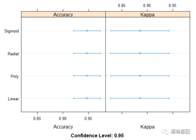
结果解读
从不同角度比较四种 SVM方法的准确性,结果显示线性(linear)的SVM在做乳腺癌的诊断中表现突出,准确率高达0.947,而上期我们选择KNN以及KKNN的算法,分别为0.9294,0.9471,从这个结果中选用加权K-邻近算法,还是SVM的准确性不分伯仲,都可以,这也就是为什么乳腺癌这个选择KNN的方法其中一个原因,自己测试一下数据觉得还是蛮有意思,后面也会继续使用机器学习的办法继续做乳腺癌的这套数据,探索哪种方法能够更好的提高诊断的准确性。
1.比较每种方法的准确性及置信区间,如下:
acc <- resamples(list(Linear = svmLinear, Poly = svmPoly, Sigmoid = svmSigmoid, Radial = svmRadial))

dotplot(acc)
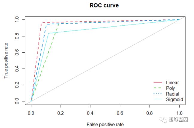
2. 绘制ROC曲线
将四种不同方法绘制在同一张图上,其中,Poly 与 Sigmoid 曲线非常接近,所以 sigmoid 使用细线,并且是实线,如下:
library(ROSE)
roc.curve(Linear.predict, test_data$diagnosis, main = "ROC curve ", col = 2, lwd = 2,
    lty = 2)
## Area under the curve (AUC): 0.947
roc.curve(Poly.predict, test_data$diagnosis, main = "ROC curve ", add = TRUE, col = 3,
    lwd = 2, lty = 2)
## Area under the curve (AUC): 0.883
roc.curve(Radial.predict, test_data$diagnosis, main = "ROC curve ", add = TRUE, col = 4,
    lwd = 2, lty = 2)
## Area under the curve (AUC): 0.920
roc.curve(Sigmoid.predict, test_data$diagnosis, main = "ROC curve ", add = TRUE,
    col = 5, lwd = 1, lty = 1)
## Area under the curve (AUC): 0.858
legend("bottomright", c("Linear", "Poly", "Radial", "Sigmoid"), col = 2:5, lty = c(1:3,
    1), lwd = c(2, 2, 2, 1), bty = "n")
References:
- Byvatov, E. and Schneider, G., 2003. Support vector machine applications in bioinformatics. Applied bioinformatics, 2(2), pp.67-77.