第3章 Python 数字图像处理(DIP) - 灰度变换与空间滤波1 - 灰度变换和空间滤波基础、Sigmoid激活函数

本节的目标

• 了解空间域图像处理的意义，以及它与变换域图像处理的区别
• 熟悉灰度变换所有的主要技术
• 了解直方图的意义以及如何操作直方图来增强图像
• 了解空间滤波的原理

import sys
import numpy as np
import cv2
import matplotlib 
import matplotlib.pyplot as plt
import PIL
from PIL import Image

print(f"Python version: {sys.version}")
print(f"Numpy version: {np.__version__}")
print(f"Opencv version: {cv2.__version__}")
print(f"Matplotlib version: {matplotlib.__version__}")
print(f"Pillow version: {PIL.__version__}")

Python version: 3.6.12 |Anaconda, Inc.| (default, Sep  9 2020, 00:29:25) [MSC v.1916 64 bit (AMD64)]
Numpy version: 1.16.6
Opencv version: 3.4.1
Matplotlib version: 3.3.2
Pillow version: 8.0.1

def normalize(mask):
    return (mask - mask.min()) / (mask.max() - mask.min() + 1e-5)

背景

灰度变换和空间滤波基础

$$g(x,y)=T[f(x,y)]\text{\hspace{1em}(3.1)}$$

式中$f(x,y)$是输入图像， $g(x,y)$是输出图像，$T$是在点$(x,y)$的一个邻域上定义的针对f的算子。

最小的邻域大小为$1\times 1$
则式(3.1)中的$T$称为灰度（也称灰度级或映射）变换函数，简写为如下：
$$s=T(r)\text{\hspace{1em}(3.2)}$$

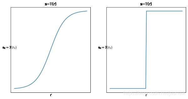
对比度拉伸

• 通过将$k$以下的灰度级变暗，并将高于$k$的灰度级变亮，产生比原图像对比度更高的一幅图像

阈值处理函数

• 小于$k$的处理为0，大于$k$的设置为1，产生一幅二级（二值）图像

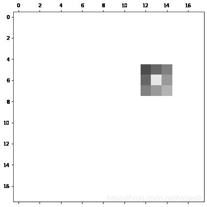
# 显示一个图像的3x3邻域
height, width = 18, 18
img_ori = np.ones([height, width], dtype=np.float)

# 图像3x3=9个像素赋了不同的值，以便更好的显示
kernel_h, kernel_w = 3, 3
img_kernel = np.zeros([kernel_h, kernel_w], dtype=np.float)
for i in range(img_kernel.shape[0]):
    for j in range(img_kernel.shape[1]):
        img_kernel[i, j] = 0.3 + 0.1 * i + 0.1 * j
img_kernel[kernel_h//2, kernel_w//2] = 0.9

img_ori[5:5+kernel_h, 12:12+kernel_w] = img_kernel

fig = plt.figure(figsize=(7, 7), num='a')
plt.matshow(img_ori, fignum='a', cmap='gray', vmin=0, vmax=1)
plt.show()

为什么会把Sigmoid函数写在这里

从Sigmoid函数的图像曲线来看，与分段线性函数的曲线类似，所以在一定程度上可以用来代替对比度拉伸，这样就不需要输入太多的参数。当然，有时可能也得不到想要的结果，需要自己多做实验。

sigmoid函数也是神经网络用得比较多的一个激活函数。

def sigmoid(x, scale):
    """
    simgoid fuction, return ndarray value [0, 1]
    param: input x: array like 
    param: input scale: scale of the sigmoid fuction, if 1, then is original sigmoid fuction, if < 1, then the values between 0, 1
    will be less, if scale very low, then become a binary fuction; if > 1, then the values between 0, 1 will be more, if scale
    very high then become a y = x
    """
    y = 1 / (1 + np.exp(-x / scale))
    return y

# sigmoid fuction plot
x = np.linspace(0, 10, 100)
x1 = x - x.max() / 2        # Here shift the 0 to the x center, here is 5, so x1 = [-5,  5]
t_stretch = sigmoid(x1, 1)
t_binary = sigmoid(x1, 0.001)

plt.figure(figsize=(10, 5))
plt.subplot(121), plt.plot(x, t_stretch), plt.title('s=T(r)'), plt.ylabel('$s_0 = T(r_0)$', rotation=0)
plt.xlabel('r'), plt.xticks([]), plt.yticks([])
plt.subplot(122), plt.plot(x, t_binary), plt.title('s=T(r)'), plt.ylabel('$s_0 = T(r_0)$', rotation=0)
plt.xlabel('r'), plt.xticks([]), plt.yticks([])
plt.tight_layout
plt.show()