深度学习评价指标总结及代码实现

1.分类任务
混淆矩阵
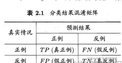
混淆矩阵就是统计分类模型的分类结果，即：统计归对类，归错类的样本的个数，然后把结果放在一个表里展示出来，这个表就是混淆矩阵。
初步理解混淆矩阵，当以二分类混淆矩阵作为入门，多分类混淆矩阵都是以二分类为基础作为延伸的！
对于二分类问题，将类别1称为正例（Positive），类别2称为反例（Negative），分类器预测正确记作真（True），预测错误记作（False），由这4个基本术语相互组合，构成混淆矩阵的4个基础元素，为：

TP（True Positive）：真正例，模型预测为正例，实际是正例（模型预测为类别1，实际是类别1）
FP（False Positive）：假正例，模型预测为正例，实际是反例 （模型预测为类别1，实际是类别2）
FN（False Negative）：假反例，模型预测为反例，实际是正例 （模型预测为类别2，实际是类别1）
TN（True Negative）：真反例，模型预测为反例，实际是反例 （模型预测为类别2，实际是类别2）

评价指标

import numpy as np
from sklearn.metrics import confusion_matrix, accuracy_score, precision_score, recall_score, f1_score, multilabel_confusion_matrix
np.seterr(divide='ignore',invalid='ignore')

"""
ConfusionMetric
Mertric   P    N
P        TP    FN
N        FP    TN
"""
class ClassifyMetric(object):
    def __init__(self, numClass, labels=None):
        self.labels = labels
        self.numClass = numClass
        self.confusionMatrix = np.zeros((self.numClass,)*2)
        
    def genConfusionMatrix(self, y_true, y_pred):
    	  return confusion_matrix(y_true, y_pred, labels=self.labels)
      
    def addBatch(self, y_true, y_pred):
        assert  np.array(y_true).shape == np.array(y_pred).shape
        self.confusionMatrix += self.genConfusionMatrix(y_true, y_pred)
 
    def reset(self):
        self.confusionMatrix = np.zeros((self.numClass, self.numClass))

    def accuracy(self):
    	  accuracy = np.diag(self.confusionMatrix).sum() / self.confusionMatrix.sum()
    	  return accuracy

    def precision(self):
    	  precision = np.diag(self.confusionMatrix) / self.confusionMatrix.sum(axis=0)
    	  return np.nan_to_num(precision)

    def recall(self):
    	  recall = np.diag(self.confusionMatrix) / self.confusionMatrix.sum(axis=1)
    	  return recall

    def f1_score(self):
    	  precision = self.precision()
    	  recall = self.recall()
    	  f1_score = 2 * (precision*recall) / (precision+recall)
    	  return np.nan_to_num(f1_score)

if __name__ == '__main__':
    y_true = ["cat", "ant", "cat", "cat", "ant", "bird"]
    y_pred = ["ant", "ant", "cat", "cat", "ant", "cat"]
    metric = ClassifyMetric(3, ["ant", "bird", "cat"])
    metric.addBatch(y_true, y_pred)
    acc = metric.accuracy()
    precision = metric.precision()
    recall = metric.recall()
    f1Score = metric.f1_score()
    print('acc is : %f' % acc)
    print('precision is :', precision)
    print('recall is :', recall)
    print('f1_score is :', f1Score)

    print('\n')
    # 与 sklearn 对比

    metric = confusion_matrix(y_true, y_pred, labels=["ant", "bird", "cat"])
    accuracy_score1 = accuracy_score(y_true, y_pred)
    print("accuracy_score", accuracy_score1)
    precision_score1 = precision_score(y_true, y_pred, average=None, zero_division=0)
    print("precision_score", precision_score1)
    recall_score1 = recall_score(y_true, y_pred, average=None, zero_division=0)
    print("recall_score", recall_score1)
    f1_score1 = f1_score(y_true, y_pred, average=None)
    print("f1_score", f1_score1)

2.语义分割
语义分割是像素级别的分类，其常用评价指标：

像素准确率（Pixel Accuracy，PA）、
类别像素准确率（Class Pixel Accuray，CPA）、
类别平均像素准确率（Mean Pixel Accuracy，MPA）、
交并比（Intersection over Union，IoU）、
平均交并比（Mean Intersection over Union，MIoU），
频率加权交并比（frequency Weighted Intersection over Union，FWIoU）

其计算都是建立在混淆矩阵（Confusion Matrix）的基础上。因此，了解基本的混淆矩阵知识对理解上述6个常用评价指标是很有益处的！
混淆矩阵
语义分割中的混淆矩阵，其关注的重点不在类别，而在像素点，判断一个像素点是否预测正确。
语义分割混淆矩阵的计算公式：

def generate_matrix(label_true, label_pred, n_class):
    mask = (label_true >= 0) & (label_true < n_class)
    label = n_class * label_true[mask] + label_pred[mask]
    confusionMatrix = np.bincount(label, minlength=n_class**2).reshape(n_class, n_class)
    return confusionMatrix

对代码进行详细解析：

label_true = np.array([
	[0,1,1],
	[2,1,0],
	[2,2,1]])
label_pred = np.array([
	[0,2,0],
	[2,1,0],
	[1,2,1]])

n = 3
mask = (label_true >= 0) & (label_true < n)
print(mask, '\n')
"""
这一句是为了保证标记的正确性（标记的每个元素值在[0, n_class）内），标记正确得到的mask是一个全为true的数组
[[ True  True  True]
 [ True  True  True]
 [ True  True  True]] 
"""

a = label_true[mask].astype(int)
print(a, '\n')
# 将label_true展平  [0 1 1 2 1 0 2 2 1] 

b = label_pred[mask]
print(b, '\n')
# 将label_pred展平  [0 2 0 2 1 0 1 2 1] 

c = n * a + b
print(c, '\n')
# [0 5 3 8 4 0 7 8 4] 

d = np.bincount(c, minlength=n**2)
print(d, '\n')
# [2 0 0 1 2 1 0 1 2] 

"""
- minlength=n_class ** 2 参数是为了保证输出向量的长度为n_class * n_class。
- 根据np.bincout的特性，c中元素的每一个值是为d中以其值为index的元素+1，
  也就是说c中元素的值其实是对应与d的index，d里面的元素，就是c中元素出现的次数，
  比如d[4]，这个4表示的就是c中的元素4，d[4] = 2，表示在c中4出现了两次，
  而c中的4是怎么得来的呢？是 a*n + b 得来的
"""

D = d.reshape(n,n)
print(D, '\n')
"""
通过reshape(n, n)将向量d转换为3*3的矩阵，其结果如下表:
[2 0 0]
[1 2 1]
[0 1 2]

则D[i,j]的值就是原来的d[i*n+j]的值，D[i,j]的值表示i*n+j在c中出现的次数，c = a*n + b，
所以就可以看出来，i 对应的就是 a，j 对应的就是 b，且它们在a与b相同的位置处，恰好代表了真实类别与预测类别，
即D[i,j]代表了预测结果为类别 j，实际标签为类别 i 的所有像素点的数目。
D[1,1]=d[1*3+1]=d[4]=2,表示预测类别为1，实际标签也为1的所有像素点数目为2。
"""

评价指标

import numpy as np
import itertools
import matplotlib.pyplot as plt
from sklearn.metrics import confusion_matrix

"""
ConfusionMetric
Mertric   P    N
P        TP    FN
N        FP    TN
"""
class SegmentationMetric(object):
    def __init__(self, numClass):
        self.numClass = numClass
        self.confusionMatrix = np.zeros((self.numClass,)*2)
        
    def genConfusionMatrix(self, imgLabel, imgPredict):
        mask = (imgLabel >= 0) & (imgLabel < self.numClass)
        label = self.numClass * imgLabel[mask] + imgPredict[mask]
        count = np.bincount(label, minlength=self.numClass**2)
        confusionMatrix = count.reshape(self.numClass, self.numClass)
        return confusionMatrix
      
    def addBatch(self, imgLabel, imgPredict):
        assert  imgLabel.shape == imgPredict.shape
        self.confusionMatrix += self.genConfusionMatrix(imgLabel, imgPredict)
 
    def reset(self):
        self.confusionMatrix = np.zeros((self.numClass, self.numClass))

    def plot_confusion_matrix(self, classes, normalize=False, title='Confusion matrix', cmap=plt.cm.Blues):
        cm = self.confusionMatrix
        if normalize:
            cm = cm.astype('float') / cm.sum(axis=1)[:, np.newaxis]
            print("Normalized confusion matrix")
        else:
            print('Confusion matrix, without normalization')
     
        plt.imshow(cm, interpolation='nearest', cmap=cmap)
        plt.title(title)
        plt.colorbar()
        tick_marks = np.arange(len(classes))
        plt.xticks(tick_marks, classes, rotation=45)
        plt.yticks(tick_marks, classes)
     
        thresh = cm.max() / 2.
        for i, j in itertools.product(range(cm.shape[0]), range(cm.shape[1])):
            num = '{:.2f}'.format(cm[i, j]) if normalize else int(cm[i, j])
            plt.text(j, i, num,
                     verticalalignment='center',
                     horizontalalignment="center",
                     color="white" if num > thresh else "black")
     
        plt.tight_layout()
        plt.ylabel('True label')
        plt.xlabel('Predicted label')
        plt.show()

    # 评价指标
      
    def pixelAccuracy(self):
        # return all class overall pixel accuracy
        #  PA = acc = (TP + TN) / (TP + TN + FP + TN)
        acc = np.diag(self.confusionMatrix).sum() /  self.confusionMatrix.sum()
        return acc
 
    def classPixelAccuracy(self):
        # return each category pixel accuracy(A more accurate way to call it precision)
        # acc = (TP) / TP + FP
        classAcc = np.diag(self.confusionMatrix) / self.confusionMatrix.sum(axis=0)
        return classAcc # 返回的是一个列表值，如：[0.90, 0.80, 0.96]，表示类别1 2 3各类别的预测准确率
 
    def meanPixelAccuracy(self):
        classAcc = self.classPixelAccuracy()
        meanAcc = np.nanmean(classAcc) # np.nanmean 求平均值，nan表示遇到Nan类型，其值取为0
        return meanAcc # 返回单个值，如：np.nanmean([0.90, 0.80, 0.96, nan, nan]) = (0.90 + 0.80 + 0.96）/ 3 =  0.89
      
    def intersectionOverUnion(self):
      	# Intersection = TP Union = TP + FP + FN
        # IoU = TP / (TP + FP + FN)
        intersection = np.diag(self.confusionMatrix) # 取对角元素的值，返回列表
        union = np.sum(self.confusionMatrix, axis=1) + np.sum(self.confusionMatrix, axis=0) - np.diag(self.confusionMatrix) # axis = 1表示混淆矩阵行的值，返回列表； axis = 0表示取混淆矩阵列的值，返回列表 
        IoU = intersection / union  # 返回列表，其值为各个类别的IoU
        return IoU
      
    def meanIntersectionOverUnion(self):
        IoU = self.intersectionOverUnion()
        mIoU = np.nanmean(IoU) # 求各类别IoU的平均
        return mIoU
 
    def frequencyWeightedIntersectionOverUnion(self):
        # FWIOU = [(TP+FN)/(TP+FP+TN+FN)]*[TP/(TP+FP+FN)]
        freq = np.sum(self.confusionMatrix, axis=1) / np.sum(self.confusionMatrix)
        iu = self.intersectionOverUnion()
        FWIoU = (freq[freq > 0] * iu[freq > 0]).sum()
        return FWIoU


if __name__ == '__main__':
    label_true = np.array([0, 1, 1, 2, 1, 0, 2, 2, 1]) # 可直接换成标注图片
    label_pred = np.array([0, 2, 0, 2, 1, 0, 1, 2, 1]) # 可直接换成预测图片
    metric = SegmentationMetric(3) # 3表示有3个分类，有几个分类就填几
    metric.addBatch(label_true, label_pred)
    print(metric.confusionMatrix)
    pa = metric.pixelAccuracy()
    cpa = metric.classPixelAccuracy()
    mpa = metric.meanPixelAccuracy()
    IoU = metric.intersectionOverUnion()
    mIoU = metric.meanIntersectionOverUnion()
    FWIoU = metric.frequencyWeightedIntersectionOverUnion()
    print('pa is : %f' % pa)
    print('cpa is :', cpa)
    print('mpa is : %f' % mpa)
    print('IoU is :', IoU)
    print('mIoU is : %f' % mIoU)
    print('FWIoU is : %f' % FWIoU)
    # metric.plot_confusion_matrix(classes=['background', 'cat', 'dog'])

    # 对比sklearn
    metric = confusion_matrix(label_true, label_pred)
    print(metric)

3.ROC曲线与AUC指标
以上的准确率Accuracy，精确度Precision，召回率Recall，F1 score，混淆矩阵都只是一个单一的数值指标，如果想观察分类算法在不同的参数下的表现情况，就可以使用一条曲线，即ROC曲线，全称为receiver operating characteristic。

ROC曲线可以用于评价一个分类器在不同阈值下的表现情况。在ROC曲线中，每个点的横坐标是false positive rate(FPR)，纵坐标是true positive rate(TPR)，描绘了分类器在True Positive和False Positive间的平衡，两个指标的计算如下：

TPR=TP/(TP+FN)，代表分类器预测的正类中实际正实例占所有正实例的比例。

FPR=FP/(FP+TN)，代表分类器预测的正类中实际负实例占所有负实例的比例，FPR越大，预测正类中实际负类越多。

ROC曲线通常如下：

其中有4个关键的点：

点(0,0)：FPR=TPR=0，分类器预测所有的样本都为负样本；

点(1,1)：FPR=TPR=1，分类器预测所有的样本都为正样本；

点(0,1)：FPR=0, TPR=1，此时FN＝0且FP＝0，所有的样本都正确分类；

点(1,0)：FPR=1，TPR=0，此时TP＝0且TN＝0，最差分类器，避开了所有正确答案。

ROC曲线相对于PR曲线有个很好的特性：

当测试集中的正负样本的分布变化的时候，ROC曲线能够保持不变，即对正负样本不均衡问题不敏感。比如负样本的数量增加到原来的10倍，TPR不受影响，FPR的各项也是成比例的增加，并不会有太大的变化。所以不均衡样本问题通常选用ROC作为评价标准。

ROC曲线越接近左上角，该分类器的性能越好，若一个分类器的ROC曲线完全包住另一个分类器，那么可以判断前者的性能更好。

如果想通过两条ROC曲线来定量评估两个分类器的性能，就可以使用AUC指标。

AUC（Area Under Curve**）为ROC曲线下的面积**，它表示的就是一个概率，这个面积的数值不会大于1。随机挑选一个正样本以及一个负样本，AUC表征的就是有多大的概率，分类器会对正样本给出的预测值高于负样本，当然前提是正样本的预测值的确应该高于负样本。

predict = [0.9,0.8,0.7,0.6,0.55,0.54,0.53,0.52,0.51,0.505,0.4,0.39,0.38,0.37,0.36,0.35,0.34,0.33,0.3,0.1];
ground_truth = [1,1,0,1,1,1,0,0,1,0,1,0,1,0,0,0,1,0,1,0];
auc = plot_roc(predict,ground_truth)

function auc = plot_roc(predict,ground_truth)
pos_num = sum(ground_truth==1);
neg_num = sum(ground_truth==0);

m = size(ground_truth,2);
[pre,Index] = sort(predict);
ground_truth = ground_truth(Index);
x = zeros(m+1,1);
y = zeros(m+1,1);
auc = 0;
x(1) = 1; y(1) = 1; %当阈值为0.1时，都被分类为了正类，所以真阳率和假阳率都为1.
for i = 2:m
    TP = sum(ground_truth(i:m) == 1); %大于x(i)的标签为1的都是真阳，大于x(i)的标签为0的都是假阳
    FP = sum(ground_truth(i:m) == 0);
    x(i) = FP/neg_num;
    y(i) = TP/pos_num;
    auc = auc + (y(i)+y(i-1))*(x(i-1)-x(i))/2;
end

x(m+1) = 0; y(m+1) = 0;
auc = auc + y(m)*x(m)/2;%这句多余
plot(x,y);
end