17_2Representation Learning and Generative Learning Deep Convolutional_Progressive Growing Style GAN

17_Representation Tying权重 CNN RNN denoising Sparse Autoencoder_潜在loss_accuracy_TSNE_KL Divergence_L1_hasing Autoencoders : https://blog.csdn.net/Linli522362242/article/details/116576478

cp17_GAN for Synthesizing Data_fully connected layer 2 convolutional_colab_ax.transAxes_twiny_spine : https://blog.csdn.net/Linli522362242/article/details/116565829

cp17_2GAN for Synthesizing_upsample_Transposed_Batch normalization_DCGAN(transposed convolution in GAN)_KL_JS divergence_双轴_EM_tape : https://blog.csdn.net/Linli522362242/article/details/117370337

Generative Adversarial Networks

     Generative adversarial networks were proposed in a 2014 paper(Ian Goodfellow et al., “Generative Adversarial Nets,” Proceedings of the 27th International Conference on Neural
Information Processing Systems 2 (2014): 2672–2680.) by Ian Goodfellow et al., and although the idea got researchers excited almost instantly, it took a few years to overcome some of the difficulties of training GANs. Like many great ideas, it seems simple in hindsight事后诸葛亮: make neural networks compete against each other in the hope that this competition will push them to excel. As shown in Figure 17-15, a GAN is composed of two neural networks:

• Generator
  
       Takes a random distribution as input (typically Gaussian) and outputs some data—typically, an image. You can think of the random inputs as the latent representations (i.e., codings) of the image to be generated. So, as you can see, the generator offers the same functionality as a decoder in a variational autoencoder, and it can be used in the same way to generate new images (just feed it some Gaussian noise, and it outputs a brand-new image). However, it is trained very differently, as we will soon see.
   
• Discriminator
  
       Takes either a fake image from the generator or a real image from the training set as input, and must guess whether the input image is fake or real.

Figure 17-15. A generative adversarial network

     During training, the generator and the discriminator have opposite goals: the discriminator tries to tell fake images from real images, while the generator tries to produce images that look real enough to trick the discriminator. Because the GAN is composed of two networks with different objectives, it cannot be trained like a regular neural network. Each training iteration is divided into two phases:

• • In the first phase, we train the discriminator. A batch of real images is sampled from the training set and is completed with an equal number of fake images produced by the generator. The labels are set to 0 for fake images and 1 for real images, and the discriminator is trained on this labeled batch for one step, using the binary cross-entropy loss. Importantly, backpropagation only optimizes the weights of the discriminator during this phase.
   
• • In the second phase, we train the generator. We first use it to produce another batch of fake images, and once again the discriminator is used to tell whether the images are fake or real. This time we do not add real images in the batch, and all the labels are set to 1 (real): in other words, we want the generator to produce images that the discriminator will (wrongly) believe to be real! Crucially, the weights of the discriminator are frozen during this step, so backpropagation only affects the weights of the generator.

     The generator never actually sees any real images, yet it gradually learns to produce convincing fake images! All it gets is the gradients flowing back through the discriminator. Fortunately, the better the discriminator gets, the more information about the real images is contained in these secondhand gradients, so the generator can make significant progress.

     Let’s go ahead and build a simple GAN for Fashion MNIST.

     First, we need to build the generator and the discriminator. The generator is similar to an autoencoder’s decoder, and the discriminator is a regular binary classifier (it takes an image as input and ends with a Dense layer containing a single unit and using the sigmoid activation function). For the second phase of each training iteration, we also need the full GAN model containing the generator followed by the discriminator:

import numpy as np
import tensorflow as tf

np.random.seed(42)
tf.random.set_seed(42)

codings_size=30

generator = keras.models.Sequential([
  keras.layers.Dense( 100, activation="selu", input_shape=[codings_size] ),
  keras.layers.Dense( 150, activation="selu" ),
  keras.layers.Dense( 28*28, activation="sigmoid"),
  keras.layers.Reshape([28,28])                                   
])

discriminator = keras.models.Sequential([
  keras.layers.Flatten( input_shape=[28,28] ),
  keras.layers.Dense( 150, activation="selu" ),
  keras.layers.Dense( 100, activation="selu" ),
  keras.layers.Dense( 1, activation="sigmoid" )                                       
])

gan = keras.models.Sequential([ generator, discriminator ])

     Next, we need to compile these models. As the discriminator is a binary classifier, we can naturally use the binary cross-entropy loss. The generator will only be trained through the gan model, so we do not need to compile it at all. The gan model is also a binary classifier, so it can use the binary cross-entropy loss. Importantly, the discriminator should not be trained during the second phase, so we make it non-trainable before compiling the gan model:

discriminator.compile( loss="binary_crossentropy", optimizer="rmsprop" )

discriminator.trainable = False
gan.compile( loss="binary_crossentropy", optimizer="rmsprop" )

     The trainable attribute is taken into account by Keras only when compiling a model, so after running this code, the discriminator is trainable if we call its fit() method or its train_on_batch() method (which we will be using), while it is not trainable when we call these methods on the gan model.

     Since the training loop is unusual, we cannot use the regular fit() method. Instead, we will write a custom training loop. For this, we first need to create a Dataset to iterate through the images:

from tensorflow import keras

(X_train_full, y_train_full), (X_test, y_test) = keras.datasets.fashion_mnist.load_data()

X_train_full = X_train_full.astype( np.float32 )/255
X_test = X_test.astype( np.float32 )/255
X_train, X_valid = X_train_full[:-5000], X_train_full[-5000:]
y_train, y_valid = y_train_full[:-5000], y_train_full[-5000:]

batch_size = 32
dataset = tf.data.Dataset.from_tensor_slices( X_train ).shuffle( 1000 )
dataset = dataset.batch( batch_size, drop_remainder=True ).prefetch(1)

import matplotlib.pyplot as plt

def plot_multiple_images( images, n_cols=None ):
  n_cols = n_cols or len(images)
  n_rows = ( len(images)-1 )//n_cols + 1
  if images.shape[-1] == 1:
    images = np.squeeze( images, axis=-1 )
    
  plt.figure( figsize=(n_cols, n_rows) )
  for index, image in enumerate(images):
    plt.subplot( n_rows, n_cols, index+1 )
    plt.imshow( image, cmap="binary" )
    plt.axis("off")

 We are now ready to write the training loop. Let’s wrap it in a train_gan() function.
https://blog.csdn.net/Linli522362242/article/details/116565829

As discussed earlier, you can see the two phases at each iteration:

• • In 1st phase, we feed Gaussian noise to the generator to produce fake images( ̂ = () ),
  and we complete this batch by concatenating an equal number of real images. The targets y1 are set to 0 for fake images and 1 for real images.
  Then we train the discriminator on this batch. Note that we set the discriminator’s trainable attribute to True: this is only to get rid of a warning that Keras displays when it notices that trainable is now False but was True when the model was compiled (or vice versa).
• • In 2nd phase, we feed the GAN some Gaussian noise. Its generator will start by producing fake images( ̂ = () ), then the discriminator will try to guess whether these images are fake or real. We want the discriminator to believe that the fake images are real, so the targets y2 are set to 1. Note that we set the trainable attribute to False, once again to avoid a warning.

def train_gan( gan, dataset, batch_size, codings_size, n_epochs=50 ):
  # gan = keras.models.Sequential([ generator, discriminator ])
  generator, discriminator = gan.layers
  for epoch in range( n_epochs ):
    print( "Epoch {}/{}".format( epoch+1, n_epochs ) )
    for X_batch in dataset:

      # phase 1 - training the discriminator
      ######################## ̂ = () ######################## 
      noise = tf.random.normal( shape=[batch_size, codings_size] ) # mean=0.0, stddev=1.0
      generated_images = generator( noise ) # training=True

      X_fake_and_real = tf.concat( [generated_images, X_batch], 
                                   axis=0 
                                 )
                # label generated_images and X_batch
                # OR
                # tf.zeros_like(generated_images) + tf.ones_like(X_batch) 
      y1 = tf.constant( [[0.]]*batch_size + [[1.]]*batch_size ) # + is tf.concat
      discriminator.trainable=True ########
      discriminator.train_on_batch( X_fake_and_real, 
                                    y1 ) # Runs a single gradient update on a single batch of data.

      # phase 2 - training the generator
      noise = tf.random.normal( shape=[batch_size, codings_size ] )
      # for training the generator, we swap the labels of real and fake examples
      # by assigning label 1 to the outputs of the generator
      y2 = tf.constant( [[1.]] * batch_size )
      discriminator.trainable = False ########
      gan.train_on_batch( noise, y2 )

    plot_multiple_images( generated_images, 8 )
    plt.show()

train_gan(gan, dataset, batch_size, codings_size, n_epochs=1)

Figure 17-16. Images generated by the GAN after one epoch of training

     That’s it! If you display the generated images (see Figure 17-16), you will see that at the end of the first epoch, they already start to look like (very noisy) Fashion MNIST images.

tf.random.set_seed(42)
np.random.seed(42)

noise = tf.random.normal( shape=[batch_size, codings_size] )
generated_images = generator( noise )
plot_multiple_images( generated_images, 8 )

 

     Unfortunately, the images never really get much better than that, and you may even find epochs where the GAN seems to be forgetting what it learned. Why is that? Well, it turns out that training a GAN can be challenging. Let’s see why.

The Difficulties of Training GANs

     During training, the generator and the discriminator constantly try to outsmart each other, in a zero-sum game. As training advances, the game may end up in a state that game theorists call a Nash equilibrium纳什均衡, named after the mathematician John Nash: this is when no player would be better off changing their own strategy, assuming the other players do not change theirs. For example, a Nash equilibrium is reached when everyone drives on the left side of the road: no driver would be better off being the only one to switch sides. Of course, there is a second possible Nash equilibrium: when everyone drives on the right side of the road. Different initial states and dynamics may lead to one equilibrium or the other. In this example, there is a single optimal strategy once an equilibrium is reached (i.e., driving on the same side as everyone else), but a Nash equilibrium can involve multiple competing strategies (e.g., a predator[ˈpredətər]捕食者 chases its prey[preɪ]猎物, the prey tries to escape, and neither would be better off changing their strategy).

     So how does this apply to GANs? Well, the authors of the paper demonstrated that a GAN can only reach a single Nash equilibrium: that’s when the generator produces perfectly realistic images, and the discriminator is forced to guess (50% real, 50% fake). This fact is very encouraging: it would seem that you just need to train the GAN for long enough, and it will eventually reach this equilibrium, giving you a perfect generator. Unfortunately, it’s not that simple: nothing guarantees that the equilibrium will ever be reached.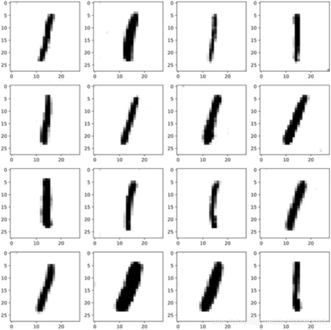
https://blog.csdn.net/Linli522362242/article/details/117370337

     The biggest difficulty is called mode collapse: this is when the generator’s outputs gradually become less diverse(OR One common cause of failure in training GANs is when the generator gets stuck in a small subspace and learns to generate similar samples. This is called mode collapse, and an example is shown in the previous figure.). How can this happen? Suppose that the generator gets better at producing convincing shoes than any other class. It will fool the discriminator a bit more with shoes, and this will encourage it to produce even more images of shoes. Gradually, it will forget how to produce anything else. Meanwhile, the only fake images that the discriminator will see will be shoes, so it will also forget how to discriminate fake images of other classes. Eventually, when the discriminator manages to discriminate the fake shoes from the real ones, the generator will be forced to move to another class. It may then become good at shirts, forgetting about shoes, and the discriminator will follow. The GAN may gradually cycle across a few classes, never really becoming very good at any of them.

     Moreover, because the generator and the discriminator are constantly pushing against each other, their parameters may end up oscillating振荡的 and becoming unstable. Training may begin properly, then suddenly diverge for no apparent reason, due to these instabilities. And since many factors affect these complex dynamics, GANs are very sensitive to the hyperparameters: you may have to spend a lot of effort fine-tuning them.

     These problems have kept researchers very busy since 2014: many papers were published on this topic, some proposing new cost functions ### For a nice comparison of the main GAN losses, check out this great GitHub project by Hwalsuk Lee. ### (though a 2018 paper ### Mario Lucic et al., “Are GANs Created Equal? A Large-Scale Study,” Proceedings of the 32nd International Conference on Neural Information Processing Systems (2018): 698–707. ### by Google researchers questions their efficiency) or techniques to stabilize training or to avoid the mode collapse issue. For example, a popular technique called experience replay consists in

• storing the images produced by the generator at each iteration in a replay buffer (gradually dropping older generated images) and
• training the discriminator using real images plus fake images drawn from this buffer (rather than just fake images produced by the current generator). This reduces the chances that the discriminator will overfit the latest generator’s outputs.

Another common technique is called mini-batch discrimination: it measures how similar images are across the batch and provides this statistic to the discriminator, so it can easily reject a whole batch of fake images that lack diversity. This encourages the generator to produce a greater variety of images, reducing the chance of mode collapse. Other papers simply propose specific architectures that happen to perform well.

     In short, this is still a very active field of research, and the dynamics of GANs are still not perfectly understood. But the good news is that great progress has been made, and some of the results are truly astounding! So let’s look at some of the most successful architectures, starting with deep convolutional GANs, which were the state of the art just a few years ago. Then we will look at two more recent (and more complex) architectures.

Deep Convolutional GANs

     The original GAN paper in 2014 experimented with convolutional layers, but only tried to generate small images. Soon after, many researchers tried to build GANs based on deeper convolutional nets for larger images. This proved to be tricky, as training was very unstable, but Alec Radford et al. finally succeeded in late 2015, after
experimenting with many different architectures and hyperparameters. They called their architecture deep convolutional GANs (DCGANs).(Alec Radford et al., “Unsupervised Representation Learning with Deep Convolutional Generative Adversarial Networks,” arXiv preprint arXiv:1511.06434 (2015).) Here are the main guidelines they proposed for building stable convolutional GANs:

• • Replace any pooling layers with strided convolutions (in the discriminator) and transposed convolutions (in the generator).
• • Use Batch Normalization in both the generator and the discriminator, except in the generator’s output layer and the discriminator’s input layer.
• • Remove fully connected hidden layers for deeper architectures.
• • Use ReLU activation in the generator for all layers except the output layer, which should use tanh.
• • Use leaky ReLU activation in the discriminator for all layers.

     These guidelines will work in many cases, but not always, so you may still need to experiment with different hyperparameters (in fact, just changing the random seed and training the same model again will sometimes work). For example, here is a small DCGAN that works reasonably well with Fashion MNIST:

The generator

• takes codings of size 100, and it projects them to 6272 dimensions (7 *7 * 128), and
• reshapes the result to get a 7 × 7 × 128 tensor.
• This tensor is batch normalized
• and fed to a transposed convolutional layer with a stride of 2, which upsamples it from 7 × 7 to 14 × 14 and reduces its depth from 128 to 64.This layer uses the selu activation function.
• The result is batch normalized again
• and fed to another transposed convolutional layer with a stride of 2, which upsamples it from 14 × 14 to 28 × 28 and reduces the depth from 64 to 1. This layer uses the tanh activation function, so the outputs will range from –1 to 1. For this reason, before training the GAN, we need to rescale the training set to that same range. We also need to reshape it to add the channel dimension:

tf.random.set_seed(42)
np.random.seed(42)

codings_size = 100

generator = keras.models.Sequential([
  keras.layers.Dense( units=7*7*128, input_shape=[codings_size,]), # ==> # 128*7*7=6272
  keras.layers.Reshape([7,7,128]),
  keras.layers.BatchNormalization(),
  # tf.keras.layers.selu(),

  keras.layers.Conv2DTranspose( 64, kernel_size=5, 
                                strides=2, padding="SAME", # (14,14,filters=64)
                                activation="selu"
                              ),
  keras.layers.BatchNormalization(),

  keras.layers.Conv2DTranspose( 1, kernel_size=5, 
                                strides=2, padding="SAME", # (28,28,filters=1)
                                activation="tanh"
                              ),                                                                 
])

generator.build()
generator.summary()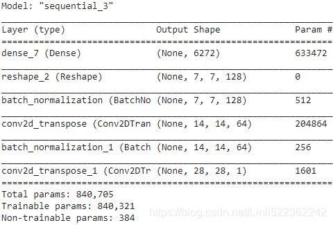

     The discriminator looks much like a regular CNN for binary classification, except instead of using max pooling layers to downsample the image, we use strided convolutions (strides=2). Also note that we use the leaky ReLU activation function.

     Overall, we respected the DCGAN guidelines, except we replaced the BatchNormalization layers in the discriminator with Dropout layers (otherwise training was unstable in this case) and we replaced ReLU with SELU in the generator. Feel free to tweak this architecture: you will see how sensitive it is to the hyperparameters (especially the relative learning rates of the two networks).

discriminator = keras.models.Sequential([
  keras.layers.Conv2D( 64, kernel_size=5, 
                       strides=2, padding="SAME",          # (14,14,filters=64)
                       activation=keras.layers.LeakyReLU(0.2),
                       input_shape=[28,28,1],
                     ),
  keras.layers.Dropout(0.4),

  keras.layers.Conv2D( 128, kernel_size=5, 
                       strides=2, padding="SAME",          # (7,7,filters=128)
                       activation=keras.layers.LeakyReLU(0.2),
                     ),
  keras.layers.Dropout(0.4),

  keras.layers.Flatten(),
  keras.layers.Dense(1, activation="sigmoid"),                                                                              
])

discriminator.build()
discriminator.summary()

gan = keras.models.Sequential([generator, discriminator])

gan.build()
gan.summary()

 The generator's last layer( transposed convolutional layer) uses the tanh activation function, so the outputs will range from –1 to 1. For this reason, before training the GAN, we need to rescale the training set to that same range. We also need to reshape it to add the channel dimension:

# scale them by a factor of 2 and shift them by –1 such that 
# the pixel intensities will be rescaled to be in the range [–1, 1]
X_train_dcgan = X_train.reshape(-1, 28,28,1)*2. -1. # reshape and rescale

     Lastly, to build the dataset, then compile and train this model, we use the exact same code as earlier.

batch_size = 32
dataset = tf.data.Dataset.from_tensor_slices( X_train_dcgan )
dataset = dataset.shuffle(1000)
dataset = dataset.batch( batch_size, drop_remainder=True ).prefetch(1)

train_gan(gan, dataset, batch_size, codings_size)

After 50 epochs of training, the generator produces images like those shown in Figure 17-17. It’s still not perfect, but many of these images are pretty convincing.
==>Figure 17-17. Images generated by the DCGAN after 50 epochs of training

Generating Fashion MNIST Images

tf.random.set_seed(42)
np.random.seed(42)

noise = tf.random.normal( shape=[batch_size, codings_size] )
generated_images = generator(noise)

plot_multiple_images( generated_images, 8)

#############################
Figure 17-18. Vector arithmetic for visual concepts (part of figure 7 from the DCGAN paper)(Reproduced with the kind authorization of the authors.)

     If you scale up this architecture and train it on a large dataset of faces, you can get fairly realistic images. In fact, DCGANs can learn quite meaningful latent representations, as you can see in Figure 17-18: many images were generated, and nine of them were picked manually (top left), including

• 3 representing men with glasses,
• 3 men without glasses, and
• 3 women without glasses.

     For each of these categories, the codings that were used to generate the images were averaged, and an image was generated based on the resulting mean codings (lower left). In short, each of the three lower-left images represents the mean of the three images located above it. But this is not a simple mean computed at the pixel level (this would result in three overlapping faces), it is a mean computed in the latent space, so the images still look like normal faces. Amazingly, if you compute men with glasses, minus men without glasses, plus women without glasses—where each term corresponds to one of the mean codings—and you generate the image that corresponds to this coding, you get the image at the center of the 3 × 3 grid of faces on the right: a woman with glasses! The eight other images around it were generated based on the same vector plus a bit of noise, to illustrate the semantic interpolation (https://blog.csdn.net/Linli522362242/article/details/117370337) capabilities of DCGANs. Being able to do arithmetic on faces feels like science fiction!

     If you add each image’s class as an extra input to both the generator and the discriminator, they will both learn what each class looks like, and thus you will be able to control the class of each image produced by the generator. This is called a conditional GAN (CGAN)(Mehdi Mirza and Simon Osindero, “Conditional Generative Adversarial Nets,” arXiv preprint arXiv:1411.1784 (2014).). ###Conditional Generative Adversarial Nets (https://arxiv.org/pdf/1411.1784.pdf) uses the class label information and learns to synthesize new images conditioned on the provided label, that is, ̃ = (|). Furthermore, conditional GANs allows us to do image-to-image translation, which is to learn how to convert a given image from a specific domain to another. In this context, one interesting work is the Pix2Pix algorithm, published in the paper Image-to-Image Translation with Conditional Adversarial Networks by PhilipIsola et al.(https://arxiv.org/pdf/1611.07004.pdf). It is worth mentioning that in the Pix2Pix algorithm, the discriminator provides the real/fake predictions for multiple patches across the image as opposed to a single prediction for an entire image.

     DCGANs aren’t perfect, though. For example, when you try to generate very large images using DCGANs, you often end up with locally convincing features but overall inconsistencies (such as shirts with one sleeve much longer than the other). How can you fix this?

Progressive Growing of GANs (PGGAN)

     An important technique was proposed in a 2018 paper(Tero Karras et al., “Progressive Growing of GANs for Improved Quality, Stability, and Variation,” Proceedings of the International Conference on Learning Representations (2018).) by Nvidia researchers Tero Karras et al.: they suggested

• generating small images at the beginning of training, 先训一个小分辨率的图像生成，训好了之后再逐步过渡到更高分辨率的图像。然后稳定训练当前分辨率，再逐步过渡到下一个更高的分辨率。
• then gradually adding convolutional layers to both the generator and the discriminator to produce larger and larger images (4 × 4, 8 × 8, 16 × 16, …, 512 × 512, 1,024 × 1,024).
• This approach resembles greedy layer-wise training of stacked autoencoders(https://blog.csdn.net/Linli522362242/article/details/116576478). 
• The extra layers get added at the end of the generator and at the beginning of the discriminator, and previously trained layers remain trainable.

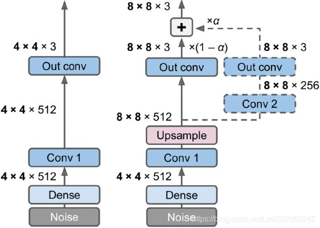     Figure 17-19. Progressively growing GAN: a GAN generator outputs 4 × 4 color images (left); we extend it to output 8 × 8 images (right)

     For example, when growing the generator’s outputs from 4 × 4 to 8 × 8 (see Figure 17-19),

• an upsampling layer (using nearest neighbor filtering) is added to the existing convolutional layer, so it outputs 8 × 8 feature maps, 
  
• which are then fed to the new convolutional layer (which uses "same" padding and strides of 1, so its outputs are also 8 × 8).
  This new layer is followed by a new output convolutional layer: this is a regular convolutional layer with kernel size 1 that projects the outputs down to the desired number of color channels (e.g., 3=rgb).
  
• To avoid breaking the trained weights of the 1st convolutional layer when the new convolutional layer(Conv 2) is added, the final output is a weighted sum of the original output layer (which now outputs 8 × 8 feature maps) and the new output layer. The weight of the new outputs is α, while the weight of the original outputs is 1 – α, and α is slowly increased from 0 to 1. In other words, the new convolutional layers (represented with dashed lines in Figure 17-19) are gradually faded in逐渐淡入, while the original output layer is gradually faded out.
   
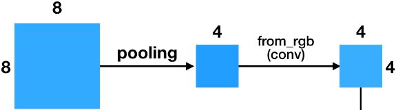
• A similar fade-in/fade-out technique is used when a new convolutional layer is added to the discriminator (followed by an average pooling layer for downsampling).
  

The paper also introduced several other techniques aimed at increasing the diversity of the outputs (to avoid mode collapse) and making training more stable:

• Minibatch standard deviation layer
  
       Added near the end of the discriminator. For each spatial position in the inputs, it computes the standard deviation across all channels and all instances in the batch ( S = tf.math.reduce_std( inputs, axis=[0, -1] ) ).
  
       These standard deviations are then averaged across all points to get a single value (v = tf.reduce_mean(S)).
  
       Finally, an extra feature map is added to each instance in the batch and filled with the computed value (

  tf.concat(  [ inputs, 
                tf.fill( [batch_size, height, width, 1], 
                         v 
                       ) 
              ],
              axis=-1
           )

  ). How does this help? Well, if the generator produces images with little variety, then there will be a small standard deviation across feature maps in the discriminator. Thanks to this layer, the discriminator will have easy access to this statistic, making it less likely to be fooled by a generator that produces too little diversity. This will encourage the generator to produce more diverse outputs, reducing the risk of mode collapse.
  我们有N个样本的feature maps(为了画图方便，不妨假设每个样本只有一个feature map OR channels=1)，我们对每个空间位置求标准差standard deviation，用numpy的std函数来说就是沿着样本的维度(feature)求std。这样就得到一张新的feature map(如果样本的feature map不止一个，那么这样构造得到的feature map数量应该是一致的)，接着feature map求平均average得到一个数。这个过程简单来说就是求mean std，作者把这个数复制成一张feature map的大小，跟原来的input feature maps 拼在一起送给Discriminator。
  
       从作者放出来的代码来看，这对应averaging=“all”的情况。作者还尝试了其他的统计量：“spatial”，“gpool”，“flat”等。它们的主要差别在于沿着哪些维度求标准差。至于它们的作用，等我的代码复现完成了会做一个测试。估计作者调参发现“all”的效果最好。
   
• Equalized learning rate均衡学习率
  
       Initializes all weights using a simple Gaussian distribution with mean 0 and standard deviation 1 rather than using He initialization. However,
       the weights are scaled down at runtime (i.e., every time the layer is executed) by the same factor as in He initialization: they are divided by , where is the number of inputs to the layer ~~.
       The paper demonstrated that this technique significantly improved the GAN’s performance when using RMSProp, Adam, or other adaptive gradient optimizers. Indeed, these optimizers normalize the gradient updates by their estimated standard deviation (see Chapter 11 https://blog.csdn.net/Linli522362242/article/details/106982127), so parameters(OR weights) that have a larger dynamic range(The dynamic range of a variable is the ratio between the highest and the lowest value it may take.) will take longer to train, while parameters with a small dynamic range may be updated too quickly, leading to instabilities. By rescaling the weights as part of the model itself rather than just rescaling them upon initialization, this approach ensures that the dynamic range is the same for all parameters, throughout training, so they all learn at the same speed. This both speeds up and stabilizes training.
  
  第二种normalization方法跟凯明大神的初始化方法[4]挂钩。He的初始化方法能够确保网络初始化的时候，随机初始化的参数不会大幅度地改变输入信号的强度。
  
       根据这个式子，我们可以推导出网络每一层的参数应该怎样初始化。可以参考pytorch提供的接口https://link.zhihu.com/?target=http%3A//pytorch.org/docs/master/nn.html%23torch-nn-init。
  
  不只是初始化的时候对参数做了调整，而是动态调整。初始化采用标准高斯分布，但是每次迭代都会对weights按照上面的式子做归一化。作者argue这样的归一化的好处在于它不用再担心参数的scale问题，起到均衡学习率的作用(Equalized learning rate)。
• Pixelwise normalization layer
  
       Added after each convolutional layer in the generator. It normalizes each activation based on all the activations in the same image and at the same location, but across all channels (dividing by the square root of the mean squared activation). In TensorFlow code, this is

  inputs / tf.sqrt( tf.reduce_mean( tf.square(X), 
                                    axis=-1, # across all channels
                                    keepdims=True
                                  ) + 1e-8
                  )

  (the smoothing term 1e-8 is needed to avoid division by zero). This technique avoids explosions in the activations due to excessive competition between the generator and the discriminator.
  
  
       从DCGAN[3]开始，GAN的网络使用batch(or instance) normalization几乎成为惯例。使用batch norm可以增加训练的稳定性，大大减少了中途崩掉的情况。作者采用了两种新的normalization方法，不引入新的参数(不引入新的参数似乎是PG-GAN各种tricks的一个卖点)。
  
       pixel norm，是local response normalization的变种。Pixel norm沿着channel维度做归一化，这样归一化的一个好处在于，activation-feature map的每个位置都具有单位长度。这个归一化策略与作者设计的Generator输出有较大关系，注意到Generator的输出层并没有Tanh或者Sigmoid激活函数，后面我们针对这个问题进行探讨。
   
• 有针对性地给样本加噪声

       通过给真实样本加噪声能够起到均衡Generator和Discriminator的作用，起到缓解mode collapse的作用，这一点在WGAN(Wasserstein GAN)的前传中就已经提到[5]。尽管使用LSGAN会比原始的GAN更容易训练，然而它在Discriminator的输出接近1的适合，梯度就消失，不能给Generator起到引导作用。针对D趋近1的这种特性，作者提出了下面这种添加噪声的方式
  
  其中，分别为第t次迭代判别器输出的修正值、第t-1次迭代真样本的判别器输出。
  从式子可以看出，当真样本的判别器输出的修正值越接近1的时候，噪声强度就越大，而输出太小(<=0.5)的时候，不引入噪声，这是因为0.5是LSGAN收敛时，D的合理输出(无法判断真假样本)，而小于0.5意味着D的能力太弱。
  官方Lasagna代码 : https://github.com/tkarras/progressive_growing_of_gans

     The combination of all these techniques allowed the authors to generate extremely convincing high-definition images of faces. But what exactly do we call “convincing”? Evaluation is one of the big challenges when working with GANs: although it is possible to automatically evaluate the diversity of the generated images, judging their quality is a much trickier and subjective task. One technique is to use human raters, but this is costly and time-consuming. So the authors proposed to measure the similarity between the local image structure of the generated images and the training images, considering every scale. This idea led them to another groundbreaking innovation: StyleGANs.

StyleGANs

     The state of the art in high-resolution image generation was advanced once again by the same Nvidia team in a 2018 paper(Tero Karras et al., “A Style-Based Generator Architecture for Generative Adversarial Networks,” arXiv preprint arXiv:1812.04948 (2018).) that introduced the popular StyleGAN architecture. The authors used style transfer techniques in the generator to ensure that the generated images have the same local structure as the training images, at every scale, greatly improving the quality of the generated images. The discriminator and the loss function were not modified, only the generator. Let’s take a look at the StyleGAN. It is composed of two networks (see Figure 17-20):
Figure 17-20. StyleGAN’s generator architecture (part of figure 1 from the StyleGAN paper)(Reproduced with the kind authorization of the authors.)

• Mapping network
  
       An 8-layer MLP that maps the latent representations z (i.e., the codings) to a vector w.
  
       This vector is then sent through multiple affine transformations (i.e., Dense layers with no activation functions, represented by the “A” boxes in Figure 17-20), which produces multiple vectors. These vectors control the style of the generated image at different levels, from fine-grained texture (e.g., hair color) to high-level features (e.g., adult or child).
  
       In short, the mapping network maps the codings to multiple style vectors.
   
• Synthesis network
  
       Responsible for generating the images. It has a constant learned input (to be clear, this input will be constant after training, but during training it keeps getting tweaked by backpropagation). It processes this input through multiple convolutional and upsampling layers, as earlier, but there are two twists:
  
       first, some noise is added to the input and to all the outputs of the convolutional layers (before the activation function).
  
       Second, each noise layer is followed by an Adaptive Instance Normalization (AdaIN) layer: it standardizes each feature map independently (by subtracting the feature map’s mean and dividing by its standard deviation),
  then it uses the style vector to determine the scale and offset of each feature map (the style vector contains one scale and one bias term for each feature map).

     The idea of adding noise independently from the codings is very important. Some parts of an image are quite random, such as the exact position of each freckle[ˈfrekl]雀斑 or hair. In earlier GANs, this randomness had to either come from the codings or be some pseudorandom noise produced by the generator itself.

• If it came from the codings, it meant that the generator had to dedicate a significant portion of the codings’ representational power to store noise: this is quite wasteful. Moreover, the noise had to be able to flow through the network and reach the final layers of the generator: this seems like an unnecessary constraint that probably slowed down training. And finally, some visual artifacts视觉伪影 may appear because the same noise was used at different levels.
   
• If instead the generator tried to produce its own pseudorandom noise, this noise might not look very convincing, leading to more visual artifacts. Plus, part of the generator’s weights would be dedicated to generating pseudorandom noise, which again seems wasteful.

By adding extra noise inputs, all these issues are avoided; the GAN is able to use the provided noise to add the right amount of stochasticity to each part of the image.

     The added noise is different for each level. Each noise input consists of a single feature map full of Gaussian noise, which is broadcast to all feature maps (of the given level) and scaled using learned per-feature scaling factors (this is represented by the “B” boxes in Figure 17-20) before it is added.

     Finally, StyleGAN uses a technique called mixing regularization (or style mixing), where a percentage of the generated images are produced using two different codings. Specifically, the codings c1 and c2 are sent through the mapping network, giving two style vectors w1 and w2. Then the synthesis network generates an image based on the styles w1 for the first levels and the styles w2 for the remaining levels.
The cutoff level is picked randomly. This prevents the network from assuming that styles at adjacent levels are correlated, which in turn encourages locality in the GAN, meaning that each style vector only affects a limited number of traits in the generated image.

     There is such a wide variety of GANs out there that it would require a whole book to cover them all. Hopefully this introduction has given you the main ideas, and most importantly the desire to learn more. If you’re struggling with a mathematical concept, there are probably blog posts out there that will help you understand it better. Then go ahead and implement your own GAN, and do not get discouraged if it has trouble learning at first: unfortunately, this is normal, and it will require quite a bit of patience before it works, but the result is worth it. If you’re struggling with an implementation detail, there are plenty of Keras or TensorFlow implementations that you can look at. In fact, if all you want is to get some amazing results quickly, then you can just use a pretrained model (e.g., there are pretrained StyleGAN models available for Keras).

In the next chapter we will move to an entirely different branch of Deep Learning: Deep Reinforcement Learning.

Exercises

1. What are the main tasks that autoencoders are used for?

• • Feature extraction : (stacked Convolutional Auto-Encoders, Denoising Autoencoders(Gaussian noise OR dropout), Sparse Autoencoders)
• • Unsupervised pretraining (Unsupervised Pretraining Using Stacked Autoencoders, Convolutional Autoencoders)
• • Dimensionality reduction(Convolutional Autoencoders, Recurrent Autoencoders)
• • Generative models (they are capable of randomly generating new data that looks very similar to the training data. For example, you could train an autoencoder on pictures of faces, and it would then be able to generate new faces. However, the generated images are usually fuzzy and not entirely realistic.)
• • Anomaly detection (an autoencoder is generally bad at reconstructing outliers)

2. Suppose you want to train a classifier, and you have plenty of unlabeled training data but only a few thousand labeled instances. How can autoencoders help? How would you proceed?

     If you want to train a classifier and you have plenty of unlabeled training data but only a few thousand labeled instances, then you could first train a deep autoencoder on the full dataset (labeled + unlabeled), then reuse its lower half for the classifier (i.e., reuse the layers up to the codings layer, included) and train the classifier using the labeled data. If you have little labeled data, you probably want to freeze the reused layers when training the classifier.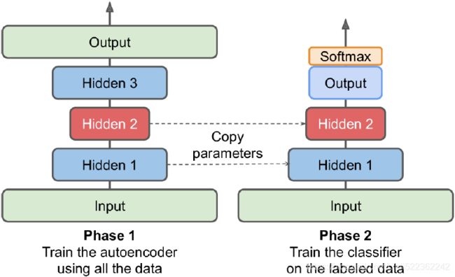
Figure 17-6. Unsupervised pretraining using autoencoders
Semi-supervised Learning : https://blog.csdn.net/Linli522362242/article/details/105973507

3. If an autoencoder perfectly reconstructs the inputs, is it necessarily a good autoencoder? How can you evaluate the performance of an autoencoder?

     The fact that an autoencoder perfectly reconstructs its inputs does not necessarily mean that it is a good autoencoder; perhaps it is simply an overcomplete autoencoder( overcomplete, where the dimensionality of the latent vector, z, is, in fact, greater than the dimensionality of the input examples (p > d). ) that learned to copy its inputs to the codings layer and then to the outputs. In fact, even if the codings layer contained a single neuron, it would be possible for a very deep autoencoder to learn to map each training instance to a different coding (e.g., the first instance could be mapped to 0.001, the second to 0.002, the third to 0.003, and so on), and it could learn “by heart” to reconstruct the right training instance for each coding. It would perfectly reconstruct its inputs without really learning any useful pattern in the data(OR without learning any useful features). In practice such a mapping is unlikely to happen, but it illustrates the fact that perfect reconstructions are not a guarantee that the autoencoder learned anything useful. However, if it produces very bad reconstructions, then it is almost guaranteed to be a bad autoencoder. To evaluate the performance of an autoencoder, one option is to measure the reconstruction loss (e.g., compute the MSE, or the mean square of the outputs minus the inputs). Again, a high reconstruction loss is a good sign that the autoencoder is bad, but a low reconstruction loss is not a guarantee that it is good. You should also evaluate the autoencoder according to what it will be used for. For example, if you are using it for unsupervised pretraining of a classifier, then you should also evaluate the classifier’s performance.

4. What are undercomplete and overcomplete autoencoders? What is the main risk of an excessively undercomplete autoencoder? What about the main risk of an overcomplete autoencoder?

     An undercomplete autoencoder is one whose codings layer is smaller than the input and output layers. If it is larger, then it is an overcomplete autoencoder.
     The main risk of an excessively undercomplete autoencoder is that it may fail to reconstruct the inputs.
     The main risk of an overcomplete autoencoder is that it may just copy the inputs to the outputs, without learning any useful features.

5. How do you tie weights in a stacked autoencoder? What is the point of doing so?

     To tie the weights of an encoder layer and its corresponding decoder layer, you simply make the decoder weights equal to the transpose of the encoder weights. This reduces the number of parameters in the model by half, often making training converge faster with less training data and reducing the risk of overfitting the training set.

     Specifically, if the autoencoder has a total of N layers (not counting the input layer), and  represents the connection weights of the  layer (e.g., layer 1 is the first hidden layer, layer N/2 is the coding layer, and layer N is the output layer), then the decoder layer weights can be defined simply as:  =  (with L = 1, 2, …, N/2).

To tie weights between layers using Keras, let’s define a custom layer:

class DenseTranspose( keras.layers.Layer ):
  def __init__( self, dense, activation=None, **kwargs ):
    self.dense = dense
    self.activation = keras.activations.get( activation )
    super().__init__( **kwargs )
 
  def build( self, batch_input_shape ):
    # for using its own bias vector
    self.biases = self.add_weight( name="bias",
                                   shape=[ self.dense.input_shape[-1] ], # uses 100 for the DenseTranspose( dense_2, activation="selu" )
                                   initializer='zeros' )
    super().build( batch_input_shape ) #batch_input_shape= (batch_size, input_dimensions)
 
  def call( self, inputs ):
    # for the DenseTranspose( dense_2, activation="selu" )
    # inputs:  Tensor("Placeholder:0", shape=(None, 30), dtype=float32)
    # self.dense.weights:  
    #           [, 
    #             # can't be used #############################################
    #           ]
    z = tf.matmul( inputs, self.dense.weights[0], 
                   transpose_b = True # for the second argument is transposed 
                 )                    # before multiplication # self.dense.weights[0] ==> (30~input features,100) # x_1*w_1 + ... + x_n*w_n + b       
    return self.activation( z+self.biases )

https://blog.csdn.net/Linli522362242/article/details/116576478 

keras.backend.clear_session()
tf.random.set_seed(42)
np.random.seed(42)
 
dense_1 = keras.layers.Dense( 100, activation="selu" ) 
dense_2 = keras.layers.Dense( 30, activation="selu" )
 
tied_encoder = keras.models.Sequential([
                                keras.layers.Flatten( input_shape=[28,28] ), # 784=28*28
                                dense_1, # weight shape: (784, 100) # input_shape(?,784 neurons)
                                dense_2, # weight shape: (100, 30)  # input_shape(?,100 neurons)                                      
               ]) # output==> (batch_size, 30)
tied_decoder = keras.models.Sequential([
                                DenseTranspose( dense_2, activation="selu" ),
                                DenseTranspose( dense_1, activation="sigmoid" ),
                                keras.layers.Reshape([28,28])
               ])
 
tied_ae = keras.models.Sequential([ tied_encoder, tied_decoder ])
 
tied_ae.compile( loss="binary_crossentropy",
                 optimizer = keras.optimizers.SGD(lr=1.5),
                 metrics=[rounded_accuracy] )
history = tied_ae.fit( X_train, X_train, epochs=10, 
                       validation_data=(X_valid, X_valid)

6. What is a generative model? Can you name a type of generative autoencoder?

     A generative model is a model capable of randomly generating outputs that resemble the training instances. For example, once trained successfully on the MNIST dataset, a generative model can be used to randomly generate realistic images of digits. The output distribution is typically similar to the training data. For example, since MNIST contains many images of each digit, the generative model would output roughly the same number of images of each digit. Some generative models can be parametrized—for example, to generate only some kinds of outputs. An example of a generative autoencoder is the variational autoencoder. https://blog.csdn.net/Linli522362242/article/details/116576478

7. What is a GAN? Can you name a few tasks where GANs can shine?

     A generative adversarial network is a neural network architecture composed of two parts, the generator and the discriminator, which have opposing objectives. The generator’s goal is to generate instances similar to those in the training set, to fool the discriminator. The discriminator must distinguish the real instances from the generated ones.

     At each training iteration, the discriminator is trained like a normal binary classifier, then the generator is trained to maximize the discriminator’s error.
( As discussed earlier, you can see the two phases at each iteration:

• • In 1st phase, we feed Gaussian noise to the generator to produce fake images( ̂ = () ),
  and we complete this batch by concatenating an equal number of real images. The targets y1 are set to 0 for fake images and 1 for real images.
  Then we train the discriminator on this batch. Note that we set the discriminator’s trainable attribute to True: this is only to get rid of a warning that Keras displays when it notices that trainable is now False but was True when the model was compiled (or vice versa).
• • In 2nd phase, we feed the GAN some Gaussian noise. Its generator will start by producing fake images( ̂ = () ), then the discriminator will try to guess whether these images are fake or real. We want the discriminator to believe that the fake images are real, so the targets-fake are set to 1. Note that we set the trainable attribute to False, once again to avoid a warning.
  
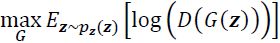
  Minimize its value with respect to the generator (G), that is,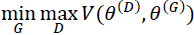 
  D is fixed, Minimize==>log(1 − (())) , suffers from vanishing gradients消失的梯度 in the early training stages( right-bottom figure,缓), The reason for this is that the outputs, G(z), early in the learning process, look nothing like real examples, and therefore D(G(z)) will be close to zero with high confidence.
  so do swap the labels of real and fake examples==>==>minimizefor using binary cross-entropy loss https://blog.csdn.net/Linli522362242/article/details/116565829

)

     GANs are used for advanced image processing tasks such as super resolution, colorization, image editing (replacing objects with realistic background), turning a simple sketch into a photorealistic image, or predicting the next frames in a video. They are also used to augment(https://blog.csdn.net/Linli522362242/article/details/108396485) a dataset (to train other models), to generate other types of data (such as text, audio, and time series), and to identify the weaknesses in other models and strengthen them.

8. What are the main difficulties when training GANs?

    Training GANs is notoriously臭名昭著 difficult, because of the complex dynamics between the generator and the discriminator. The biggest difficulty is mode collapse, where the generator produces outputs with very little diversity. Moreover, training can be terribly unstable: it may start out fine and then suddenly start oscillating摆动的 or diverging, without any apparent reason. GANs are also very sensitive to the choice of hyperparameters.

9. Exercise: Try using a denoising autoencoder to pretrain an image classifier. You can use MNIST (the simplest option), or a more complex image dataset such as CIFAR10 if you want a bigger challenge. Regardless of the dataset you're using, follow these steps:

• Split the dataset into a training set and a test set. Train a deep denoising autoencoder on the full training set.

  from tensorflow import keras
  
  [X_train, y_train], [X_test, y_test] = keras.datasets.cifar10.load_data()
  X_train = X_train /255.
  X_test = X_test / 255.

  

  X_train.shape

  

  y_train.shape

  

  import tensorflow as tf
  import numpy as np
  
  denoising_encoder = keras.models.Sequential([
    keras.layers.GaussianNoise(0.1, input_shape=[32, 32, 3]),
    keras.layers.Conv2D(32, kernel_size=3, padding="same", activation="relu"),
    keras.layers.MaxPool2D(),
    keras.layers.Flatten(), # since Dense
    keras.layers.Dense(512, activation="relu"),                                             
  ])
  
  denoising_encoder.summary()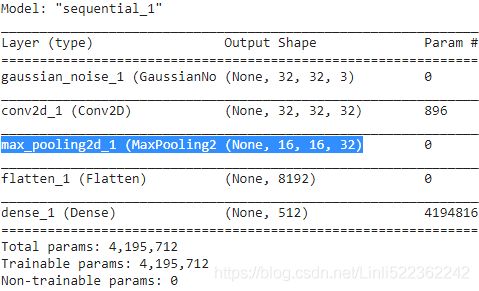

  

  denoising_decoder = keras.models.Sequential([
    keras.layers.Dense( 16*16*32, activation="relu", input_shape=[512]),
    keras.layers.Reshape([16,16,32]),
    keras.layers.Conv2DTranspose( filters=3, kernel_size=3, 
                                  strides=2, padding="same", 
                                  activation="sigmoid"
                                )                                             
  ])
  denoising_decoder.summary()

  
   When compiling the stacked autoencoder, we use the binary cross-entropy loss instead of the mean squared error. We are treating the reconstruction task as a multilabel binary classification problem(https://blog.csdn.net/Linli522362242/article/details/103866244): each pixel(or each label) intensity represents the probability that the pixel should be R/G/B. Framing it this way (rather than as a regression problem) tends to make the model converge faster.

  denoising_ae = keras.models.Sequential([denoising_encoder, denoising_decoder])
  
  denoising_ae.compile( loss="binary_crossentropy", 
                        optimizer=keras.optimizers.Nadam(),
                        metrics=["mse"]
                      )
  history = denoising_ae.fit( X_train, X_train, epochs=10,
                              validation_data=(X_test, X_test)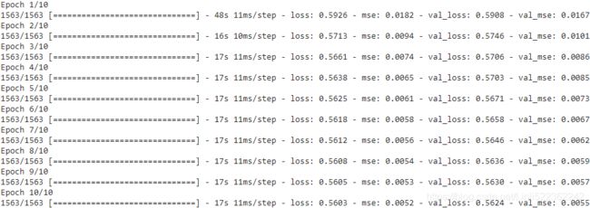
                            )

  

• Check that the images are fairly well reconstructed. Visualize the images that most activate each neuron in the coding layer.

  import matplotlib.pyplot as plt
  %matplotlib inline
  
  n_images = 5
  new_images = X_test[:n_images]
  new_images_noisy = new_images + np.random.randn( n_images, 32, 32, 3 )*0.1
  new_images_denoised = denoising_ae.predict( new_images_noisy )
  
  plt.figure( figsize=(6, n_images*2) )
  for index in range( n_images ):
    plt.subplot( n_images, 3, index*3 +1 )
    plt.imshow( new_images[index] )
    plt.axis('off')
    if index ==0:
      plt.title("Original")
    
    plt.subplot( n_images, 3, index*3 +2 )
    # if not clip: warning Clipping input data to the valid range for imshow with RGB data ([0..1] for floats or [0..255] for integers).
    plt.imshow( np.clip(new_images_noisy[index], 0., 1.) )
    plt.axis('off')
    if index ==0:
      plt.title("Noisy")
  
    plt.subplot( n_images, 3, index*3 +3 )
    plt.imshow( new_images_denoised[index] )
    plt.axis('off')
    if index ==0:
      plt.title('Denoised')
  
  plt.show()

  

• Build a classification DNN, reusing the lower layers of the autoencoder. Train it using only 500 images from the training set. Does it perform better with or without pretraining?