小武与SSD与pytorch-尝试手撕代码
参考连接:
https://zhuanlan.zhihu.com/p/33544892
https://zhuanlan.zhihu.com/p/31427288
知乎说的还是不错的、
SSD作为one-stage 和 two-stage结合的方法
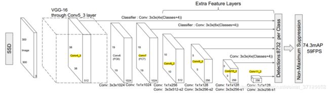
先post上SSD的流程图:
代码的实现部分:核心还是数据流:
我们跟着一张图如何走的形态,走下去看看每一步都会发生什么。同时也通过该代码学习下如何用pytorch搭建自己的网络。
开头的nn.module,torch.nn是专门为神经网络设计的模块化接口。nn构建于autograd之上,可以用来定义和运行神经网络。nn.Module是nn中十分重要的类,包含网络各层的定义及forward方法。
代码总体结构
代码的总体结构:先定义了multibox的方法,将vgg和add_extras 放入到multibox中进行处理得到新的vgg基本网络和新的额外的网络同时生成处理置信度和处理位置逻辑回顾的网络。最后一起放入到大的网络中,将刚刚生成这些网络,进行融合,并且加入了前向传播。最后是在其他部分直接调用了build_sad的方法。
    base = {
    '300': [64, 64, 'M', 128, 128, 'M', 256, 256, 256, 'C', 512, 512, 512, 'M',
            512, 512, 512],
    '512': [],
}
extras = {
    '300': [256, 'S', 512, 128, 'S', 256, 128, 256, 128, 256],
    '512': [],
}
mbox = {
    '300': [4, 6, 6, 6, 4, 4],  # number of boxes per feature map location
    '512': [],
}
    def build_ssd(phase, size=300, num_classes=21):
        if phase != "test" and phase != "train":
            print("ERROR: Phase: " + phase + " not recognized")
            return
        if size != 300:
            print("ERROR: You specified size " + repr(size) + ". However, " +
                  "currently only SSD300 (size=300) is supported!")
            return
        base_, extras_, head_ = multibox(vgg(base[str(size)], 3),
                                         add_extras(extras[str(size)], 1024),
                                         mbox[str(size)], num_classes)
                                          #融合到了multibox中给出对应的vgg,extral_layer,还有生成处理置信度和处理位置逻辑回顾的网络。最后将这些放到了SSD的总体网络中。我们这里使用了SSD300 所以size是300
        return SSD(phase, size, base_, extras_, head_, num_classes)
mutilbox部分(VGG分析,extra_layer分析)
所以我们先看看multibox,这里会生成一系列我们需要的结构:可以看到输入部分有vgg和extra_layers 还有其他的参数。我们会结合extral_layer和vgg来看看.从VGG的搭建来看和上图的模型是符合的。Conv4-3后讲全连接层替换成了33和11的卷积网络,其中conv6加了dilation=6.
来自知乎的解释:
从代码书写的角度,这一段代码非常值得借鉴,我们会发现作者重写vgg代码的时候并没有一层层的写出来,作者先是写了一个
base = {
‘300’: [64, 64, ‘M’, 128, 128, ‘M’, 256, 256, 256, ‘C’, 512, 512, 512, ‘M’, 512, 512, 512],
‘512’: [],
}
然后通过读取这个base来构建vgg网络,也就是下面的for循环 部分。通过M和C的设置巧妙的将不同的层都用一个定义的maxpooling 就可以多元化。M是要接maxpool,C是接ceil_mode为True的maxpool。而不在需要反复的写。而且layer+=的使用是的代码很简洁。 def vgg 简单的几行却将整个网络的总体部分都写完。vgg + conv6 +conv7 都有了 。
def vgg(cfg, i, batch_norm=False):
    layers = []
    in_channels = i
    for v in cfg:
        if v == 'M':
            layers += [nn.MaxPool2d(kernel_size=2, stride=2)]
        elif v == 'C':
            layers += [nn.MaxPool2d(kernel_size=2, stride=2, ceil_mode=True)]
        else:
            conv2d = nn.Conv2d(in_channels, v, kernel_size=3, padding=1)
            if batch_norm:
                layers += [conv2d, nn.BatchNorm2d(v), nn.ReLU(inplace=True)]
            else:
                layers += [conv2d, nn.ReLU(inplace=True)]
            in_channels = v
    pool5 = nn.MaxPool2d(kernel_size=3, stride=1, padding=1)
    conv6 = nn.Conv2d(512, 1024, kernel_size=3, padding=6, dilation=6)
    conv7 = nn.Conv2d(1024, 1024, kernel_size=1)
    layers += [pool5, conv6,
               nn.ReLU(inplace=True), conv7, nn.ReLU(inplace=True)]
    return layers
这里的extra部分也是用了一个
extras = {
‘300’: [256, ‘S’, 512, 128, ‘S’, 256, 128, 256, 128, 256],
‘512’: [],
}
带上循环就可以用有一句简单的代码将网络剩余的结果复现了。
我们可以发现上面的vgg部分仅写完了conv7不得分,但是我们的网络实际上还需要在做一些卷积处理,通过这样来得到不同大小的featuremap。所以通过add_extras就可以将下面的层给写完。S的部分 是指stride,通过这样的方式 来缩小featuremap 所以这里有两步是缩小了feature map是符合上图的网络结构的
def add_extras(cfg, i, batch_norm=False):
    # Extra layers added to VGG for feature scaling
    layers = []
    in_channels = i
    flag = False
    for k, v in enumerate(cfg):
        if in_channels != 'S':
            if v == 'S':
                layers += [nn.Conv2d(in_channels, cfg[k + 1],
                           kernel_size=(1, 3)[flag], stride=2, padding=1)]
            else:
                layers += [nn.Conv2d(in_channels, v, kernel_size=(1, 3)[flag])]
            flag = not flag
        in_channels = v
    return layers
最后通过mutilbox进一步的处理上面的vgg 和extra_largers,同时返回了处理featuremap得到loc_layers = [],conf_layers = []一个是用来处理位置逻辑回归的一个是用来处理类别置信度的。vgg出来的那部分的loc_layer 和conf_layers处理还不同于下面的其他的所以分开。
来自知乎的解释:

def multibox(vgg, extra_layers, cfg, num_classes):
    loc_layers = []
    conf_layers = []
    vgg_source = [21, -2]
    for k, v in enumerate(vgg_source):
        loc_layers += [nn.Conv2d(vgg[v].out_channels,
                                 cfg[k] * 4, kernel_size=3, padding=1)]
        conf_layers += [nn.Conv2d(vgg[v].out_channels,
                        cfg[k] * num_classes, kernel_size=3, padding=1)]
    for k, v in enumerate(extra_layers[1::2], 2):
        loc_layers += [nn.Conv2d(v.out_channels, cfg[k]
                                 * 4, kernel_size=3, padding=1)]
        conf_layers += [nn.Conv2d(v.out_channels, cfg[k]
                                  * num_classes, kernel_size=3, padding=1)]
    return vgg, extra_layers, (loc_layers, conf_layers)
所以上面部分完成了下面几个部分的搭建,简单的代码却可以把这些部分都给出来。巧妙的使用了for循环。也看到了pytorch的简洁。只是个个部分,但是连接的话还有下面的前向传播的代码。

import torch
import torch.nn as nn
import torch.nn.functional as F
from torch.autograd import Variable
from layers import *
from data import voc, coco
import os
class SSD(nn.Module):
    """Single Shot Multibox Architecture
    The network is composed of a base VGG network followed by the
    added multibox conv layers.  Each multibox layer branches into
        1) conv2d for class conf scores
        2) conv2d for localization predictions
        3) associated priorbox layer to produce default bounding
           boxes specific to the layer's feature map size.
    See: https://arxiv.org/pdf/1512.02325.pdf for more details.

    Args:
        phase: (string) Can be "test" or "train"
        size: input image size
        base: VGG16 layers for input, size of either 300 or 500
        extras: extra layers that feed to multibox loc and conf layers
        head: "multibox head" consists of loc and conf conv layers
    """

    def __init__(self, phase, size, base, extras, head, num_classes):
        super(SSD, self).__init__()
        self.phase = phase #输入的参数
        self.num_classes = num_classes #类别,和我们搭建的网络参数有关
        self.cfg = (coco, voc)[num_classes == 21]
        self.priorbox = PriorBox(self.cfg) #box的数目也是有关的
        self.priors = Variable(self.priorbox.forward(), volatile=True)
        self.size = size

        # SSD network
        self.vgg = nn.ModuleList(base) #vgg网络的使用
        # Layer learns to scale the l2 normalized features from conv4_3
        self.L2Norm = L2Norm(512, 20) #L2正则化的使用
        self.extras = nn.ModuleList(extras) # 额外的网络架构的输入

        self.loc = nn.ModuleList(head[0]) # 生成位置逻辑回归的网络
        self.conf = nn.ModuleList(head[1]) #生成类别置信度的网络

        if phase == 'test':
            self.softmax = nn.Softmax(dim=-1)
            self.detect = Detect(num_classes, 0, 200, 0.01, 0.45)
用pytorch的开头都是用__init__来初始化一系列参数的,这些参数在后面部分都会用到。forward 和 load_weights 都是重要方法,当我们用pytorch写代码的时候。forward可以看出我们一张图片进入到出来的结果,load_weights一般用于当我们有预训练模型训练的时候。所以在这里,我们结合前面就可以看看数据的流动了。
首先符合模型的走到了vgg,这里用了source这个主要是是用于feature map的检测部分。我们称之为source layer,总体部分继续往前走,source,layer用来做检测的分支
multibox即将选中的各个层的特征图提取出来(选中的层都在前面用黄色标出),然后对每个特征图的每个像素点预测目标box相对于default box的offsets和每个类的置信度。具体来说,如果某一层每个像素点定义k个default boxes,有num_classes个类,则该像素点总的输出个数为k(num_classes+4)。不过在代码中,网络分为2个head(loc_layers和conf_layers)分别预测位置信息和类别信息。
       def forward(self, x):
            """Applies network layers and ops on input image(s) x.

            Args:
                x: input image or batch of images. Shape: [batch,3,300,300].

            Return:
                Depending on phase:
                test:
                    Variable(tensor) of output class label predictions,
                    confidence score, and corresponding location predictions for
                    each object detected. Shape: [batch,topk,7]

                train:
                    list of concat outputs from:
                        1: confidence layers, Shap

e: [batch*num_priors,num_classes]
                    2: localization layers, Shape: [batch,num_priors*4]
                    3: priorbox layers, Shape: [2,num_priors*4]
        """
        sources = list()
        loc = list()
        conf = list()

       #第一个特征图,来自vgg的conv4_3的层
        # apply vgg up to conv4_3 relu
        for k in range(23):
            x = self.vgg[k](x)

        #第一个特征图,经过L2的归一化,然后填充到source中
        s = self.L2Norm(x)
        sources.append(s)
        #先

        # apply vgg up to fc7
        for k in range(23, len(self.vgg)):
            x = self.vgg[k](x)
        sources.append(x)

        # extra layers向前传播四个特征图
        #同时将要预测的部分继续填充到source layer 中
        # apply extra layers and cache source layer outputs
        for k, v in enumerate(self.extras):
            x = F.relu(v(x), inplace=True)
            if k % 2 == 1:
                sources.append(x)

        #将要输出的检测的部分都append进去了sourcelayer中
        # apply multibox head to source layers
        for (x, l, c) in zip(sources, self.loc, self.conf):
            loc.append(l(x).permute(0, 2, 3, 1).contiguous())
            conf.append(c(x).permute(0, 2, 3, 1).contiguous())

        loc = torch.cat([o.view(o.size(0), -1) for o in loc], 1)
        conf = torch.cat([o.view(o.size(0), -1) for o in conf], 1)
        if self.phase == "test":
            output = self.detect(
                loc.view(loc.size(0), -1, 4),                   # loc preds
                self.softmax(conf.view(conf.size(0), -1,
                             self.num_classes)),                # conf preds
                self.priors.type(type(x.data))                  # default boxes
            )
        else:
            output = (
                loc.view(loc.size(0), -1, 4),
                conf.view(conf.size(0), -1, self.num_classes),
                self.priors
            )
        return output

    def load_weights(self, base_file):
        other, ext = os.path.splitext(base_file)
        if ext == '.pkl' or '.pth':
            print('Loading weights into state dict...')
            self.load_state_dict(torch.load(base_file,
                                 map_location=lambda storage, loc: storage))
            print('Finished!')
        else:
            print('Sorry only .pth and .pkl files supported.')
代码中有一句:
for (x, l, c) in zip(sources, self.loc, self.conf):
我们知道source是不同层需要用来预测的特征图
而loc和conf是分别的用来预测置信度和预测坐标位置回归的
这里使用了zip
zip的作用:
zip() 函数用于将可迭代的对象作为参数,将对象中对应的元素打包成一个个元组,然后返回由这些元组组成的列表。
所以分别将source,loc, con对应的元素,组成元祖,将元祖组成列表。
还有一句:
loc.append(l(x).permute(0, 2, 3, 1).contiguous())
conf.append(c(x).permute(0, 2, 3, 1).contiguous())
这里处理的情况,之前在公司的CTC前面一层也有遇到过这样的处理。这里贴出来知乎的答案,和CTC当时这样处理的原因基本上一致。
将(batch_size, c , h,w)? (batch_size,h, w, c)?(batch_size,h, wc)?(batch_size,hw*c)
