Clinical grade computional pathology using weakly supervised deep learning on whole slide images

Abstract

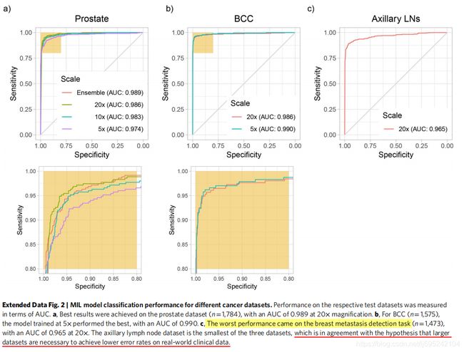
需要大量手工标注数据集一直阻碍病理学方面的决策支持系统的发展以及在临床上部署。为了解决这一问题，本文提出了基于多实例学习的深度学习系统，其仅仅使用已报告的诊断作为训练的标签，得意边广泛且费时间的逐像素手工标注。本文在来自15187位病人的44732张全切片图像构成的数据集上评估了该框架的性能，并且这些数据没有经过任何整理(curation)。前列腺癌、基底细胞癌和乳腺癌转移到腋窝淋巴结的试验结果显示，所有癌症类型的曲线下面积(areas under the curve)均在0.98以上。该系统的临床应用将使得在保持100%敏感度下病理学家能够排除65-75%的无效切片。实验结果表明，该系统能够在史无前例的大范围数据集上训练准确的分类模型，以此为临床级决策支持系统的落地奠定基础。

The development of decision support systems for pathology and their deployment in clinical practice have been hindered by the need for large manually annotated datasets. To overcome this problem, we present a multiple instance learning-based deep learning system that uses only the reported diagnoses as labels for training, thereby avoiding expensive and time-consuming pixel-wise manual annotations. We evaluated this framework at scale on a dataset of 44,732 whole slide images from 15,187 patients without any form of data curation. Tests on prostate cancer, basal cell carcinoma and breast cancer metastases to axillary lymph nodes resulted in areas under the curve above 0.98 for all cancer types. Its clinical application would allow pathologists to exclude 65–75% of slides while retaining 100% sensitivity. Our results show that this system has the ability to train accurate classification models at unprecedented scale, laying the foundation for the deployment of computational decision support systems in clinical practice.

Introduction

病理学的诊断方式百年未变，深度学习将带来变革

• 病理学是现代医学的基石，特别在癌症治疗领域。基于载玻片的病理学家的诊断是临床和组织学研究的基础，更是决定如何治疗病人的重要依据。然而，过去一个世纪，用于诊断、癌症分级分期的显微镜标准方法几乎没有改变。
• 而此时，其他医学领域，诸如放射医疗学，可计算的研究和临床应用已经有一定历史了。
• 近些年，数字病理学作为一项潜在质量标准出现，其将载玻片通过数字扫描器获得全切片图像。扫描器技术以及全切片数字图像的大量获取，推动了计算机协助诊断设备的出现，以及促进了了病理学家数字工作流程的发展。
• 而传统上，用于医疗图像分析的决策支持系统的预测模型依赖于专业的人工工程特征的提取。这些方法需要专业领域知识，并且总体来说，临床应用上的性能不好。
• 随着近几年深度学习在解决图像分类的巨大成功，其改变传统方式的决策支持系统方法。
  当前遇到的问题：数据集小，标注困难且工作量大，临床应用存疑
• 可计算病理学相较于其他领域，必须面对与病例数据生成相关的额外挑战：严重缺乏大量的标注数据集
• 当前最先进的病理数据集很小并且被严格整理过。
• 乳腺癌转移检测挑战赛CAMELYON16 Challenge包含该标注字段最大标签的数据集之一，共有400个未彻底标注的WSI全切片图像
• 在这些小数据集上的监督式分类任务应用深度学习取得了令人振奋的结果。值得注意的是，这些小数据集在鉴别良性组织和转移乳腺癌上取得了同专业病理学家相当的成绩。
• 然而这些模型在临床上的实用性仍然存有疑问，这是因为小数据集不能捕获临床样本的巨大差异性
• 为了合理定位当前计算机相关方法的缺点以及促进决策支持工具的临床部署，就需要在大规模数据集上对模型进行训练和验证，而这些大数据集则代表了临床上每天病例的广泛差异性。
• 大规模数据集上依赖于昂贵且费时的人工标注是不可能的
  本文贡献
• 通过收集大量计算机相关的病理数据集以及提出不需要像素级标注的大规模数据集上分类模型解决上述问题。
• 更进一步，依据本文的结果，相比于现有文献提出了临床适用性的新测量方法，规范了临床级决策支持系统的概念
  数据集
  计算病理学数据集：
  ①含24859切片的前列腺穿刺活检数据集
  ②含9962切片的皮肤数据集
  ③含9894切片的淋巴结的乳腺癌转移数据集
• 这些数据集中的每一个都至少比其邻域内所有其他数据集大一个数量级
• 为了将这一点与其他计算机视觉问题联系起来，我们分析了88个imagenet数据集的等效像素数。（重点是数据没有整理curation）
• 为每种组织类型收集的载玻片代表了至少一年的临床病例，因此代表了在真正的病理实验室中生成的载玻片，包括常见的伪影，如气泡、切片刀不规则、固定问题、烧灼，褶皱和裂缝，以及数字化工件，如条纹和模糊区域
• 在三种组织类型中，我们包括17661个外部载玻片，它们产生于美国和其他44个国家各自机构的病理实验室，其说明了计算病理学研究中前所未有的技术变异性。
• 所选择的数据集代表了不同但互补的临床实践观点，并提供了对灵活和健壮的决策支持系统应该能够解决的挑战类型的洞察。
  方法
• 适用切片级（slide-level）诊断来进行弱监督方式的训练分类模型。
• WSI（Whole Slide Image)分类问题是不同标准多实例假设的例子，多实例学习MIL(Multiple instance learning)已经广泛应用于包括计算机视觉在内的许多机器学习领域。
• 切片级诊断在在特定WSI的所有tile上投射弱标签，如果该切片是负样本，则其所有tiles必须是负的，说明其没有包含肿瘤；相反，如果slide是正样本，其至少包含一个正的tile，说明其包含肿瘤。
• 现有弱监督WSI分类方法都是有赖于IL多实例假设变体下训练的深度学习模型。典型的，两步走：1.tile级的MIL多实例学习训练的分类器；2.将WSI（全切片）的每个tile预测分数进行聚合，聚合通常通过将其结果与多种策略组合，或通过学习融合模型。
  利用MIL多实例学习训练深度神经网络，得到一个语义丰富的tile级特征表示，然后将这些特征表示输入RNN循环神经网络，聚合全切片信息并得到最终分类结果。

Results

测试每个组织类型的用MIL训练的ResNet34模型的性能

分类准确度的数据集尺寸依赖

特征空间到二维图像的可视化模型检查

不同切片局聚合方法的对比

MIL-RNN错误节点的病理专家分析

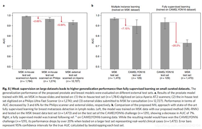
不同机构以及扫描设备引入的技术差异性研究

全监督学习与弱监督学习的比对

Method

Hardware and software

硬件：Memorial Sloan Kettering Cancer Center (MSK) 的高性能计算集群：7个NVIDIA DGX-1计算节点，每个节点包含8个V100 Volta GPU和8TB SSD，每个模型在单GPU上训练

WSI datasets

任务：
1.前列腺癌分类
2.Skin cancer basal cell carcinoma (BCC)皮肤基底细胞癌分类
3.腋淋巴乳腺癌转移检测

每个数据集分为：70%训练集，15%验证集，15%测试集
前列腺癌数据集，外部数据没有加入训练集，而是加入测试集。
而皮肤癌以及乳腺癌转移则加入训练集而非测试集。

对于前列腺癌与腋淋巴结乳腺癌转移数据集，真实标签来自实验室信息系统（Laboratory Information System， LIS），而对于皮肤基底细胞癌数据集，则通过训练有数的专家进行确认和最终手工为每个病例设置二进制标签。

数据没有整理（Curation），以此测试本文系统在真实环境中的适用性

仅当slide-level类已知而该slide内每个tile的类未知时，通过经典MIL多实例学习方法规范基于tile-level分类器的全数字切片分类。
n个slide组成的玻片池中的每个slide可作为包含多个实例的bag，每个tile为224×224大小
正样本bag至少包含一个被分类器预测为正样本的实例，而负样本则一个也不包含。
给定一个bag，所有实例被彻底分类，并根据他们是正样本的可能性进行排序。

为了解决MIL多实例学习任务，需要tile-level表示的学习，其能够将正样本slides中的可辨识的tiles与其他tiles线性分离。

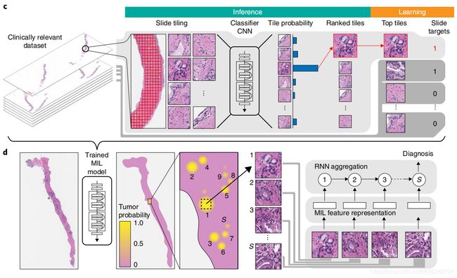
The complete pipeline for the MIL classification algorithm (Fig. 1c) comprises the following steps:
(1) tiling of each slide in the dataset (for each epoch, which consists of an entire pass through the training data);
(2) a complete inference pass through all of the data;
(3) intra-slide ranking of instances;
(4) model learning based on the top-ranked instance for each slide.

Slide tiling

将每个slide分成网格产生实例，通过OSTU大津阈值法进行背景区分，降低每个slide的可计算数量
三种放大尺寸比对：5×，10×，20×
不同放大尺寸以及重叠下进行训练和验证

放大尺寸	training&validation重叠比例	test重叠比例
5×	67%	80%
10×	50%	80%
20×	0%	80%

Bags：$B=B_{s_i}:i=1,2,...,n$
$B_{s_i}=b_{i,1},b_{i,2},...,b_{i,m}$
{% blockquote %}
Given a tiling strategy, we produce bags $B=B_{s_i}:i=1,2,...,n$, where $B_{s_i}=b_{i,1},b_{i,2},...,b_{i,m}$ is the bag for slide $s_i$ containing mi total tiles.
{% endblockquote %}

Model training

The model is a function $f\_\theta$ with current parameter $\theta$ that maps input tiles bi,j to class probabilities for ‘negative’ and ‘positive’ classes. Given our bags $B$, we obtain a list of vectors $O=o\_i:i=1,2,\dots ,n$—one for each slide $s\_i$ containing the probabilities of class ‘positive’ for each tile $b\_i,j:j=1,2,\dots ,m$ in $B\_s\_i$. We then obtain the index ki of the tile within each slide, which shows the highest probability of being ‘positive’: ki=argmax(oi).

This is the most stringent version of MIL, but we can relax the standard MIL assumption by introducing hyper-parameter $K$ and assume that at least $K$ tiles exist in positive slides that are discriminative. For $K=1$, the highest ranking tile in bag $B_{s_i}$ is then $b_i,k$. The output of the network ${\hat{y}}_i=f_{\theta }(b_i,k)$ can then be compared to $y_i$, the target of slide $s_i$, through the cross-entropy loss $l$ as in equation (1). Similarly, if $K>1$, all selected tiles from a slide share the same target $y_i$ and the loss can be computed with equation (1) for each one of the $K$ tiles:
$$l=-w1[y_{i}log[{\hat{y}}_i]]-w0[(1-y_i)log[1-{\hat{y}}_i]](1)$$

w0,w1分别是负、正类的权重
最终损失是小批量损失的加权平均
Adam优化算法，随机梯度下降
512批量-AlexNet，256批量-ResNets，128-VGG&DenseNet201
所有模型通过ImageNet预训练权重进行初始化，使用早停法避免过拟合。

Model testing

每个slide的所有tile通过神经网络，设置阈值0.5进行MIL学习
假设一个slide为正的概率是该slide中所有tile中的最高概率
tile上概率的最大池化是最简单的聚合技术

不同聚合方法的研究

朴素多尺度聚集（Naive multiscale aggregation）

5×，10×，20×下平均和最大池化获得谱图多尺度模型

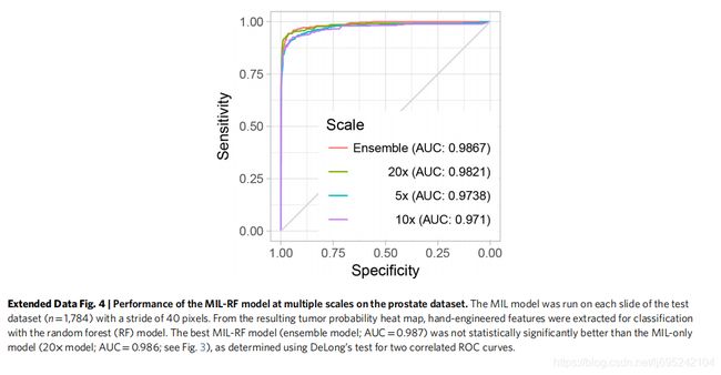
基于随机森林的玻片聚合（Random forest-based slide integration）

使用me讴歌勒种tile的数量训练逻辑回归模型，并铁架一些全局和局部特征。
在验证集上训练随机森林而非训练集，以此避免过拟合

The features extracted are:
(1) total count of tiles with probability ≥0.5;
(2–11) tenbin histogram of tile probability;
(12–30) count of connected components for a probability threshold of 0.1 of size in the ranges 1–10, 11–15, 16–20, 21–25, 26–30, 31–40, 41–50, 51–60, 61–70 and >70, respectively;
(31–40) ten-bin local histogram with a window of size 3×3 aggregated by max-pooling;
(41–50) ten-bin local histogram with a window of size 3×3 aggregated by averaging;
(51–60) ten-bin local histogram with a window of size 5×5 aggregated by max-pooling;
(61–70) ten-bin local histogram with a window of size 5×5 aggregated by averaging;
(71–80) ten-bin local histogram with a window of size 7×7 aggregated by max-pooling;
(81–90) ten-bin local histogram with a window of size 7×7 aggregated by averaging;
(91–100) ten-bin local histogram with a window of size 9×9 aggregated by max-pooling;
(101–110) ten-bin local histogram with a window of size 9×9 aggregated by averaging;
(111–120) ten-bin histogram of all tissue edge tiles;
(121–130) ten-bin local histogram of edges with a linear window of size 3×3 aggregated by max-pooling;
(131–140) ten-bin local histogram of edges with a linear window of size 3×3 aggregated by averaging;
(141–150) ten-bin local histogram of edges with a linear window of size 5×5 aggregated by max-pooling;
(151–160) ten-bin local histogram of edges with a linear window of size 5×5 aggregated by averaging;
(161–170) ten-bin local histogram of edges with a linear window of size 7×7 aggregated by max-pooling;
(171–180) ten-bin local histogram of edges with a linear window of size 7×7 aggregated by averaging.

基于RNN的玻片聚合（RNN-based slide integration）

模型：$f$
特征提取器$f_F$ 将像素空间转为表示空间
线性分类器$f_C$ 将表示变量投射为类概率

1.给定一个slide和模型f，根据正类概率得到slide中最感兴趣的S个tile的列表
向量表示的有序序列$e=e_1,e_2,...e_s$同状态向量$h$一起作为RNN输入，
step i=1,2,…,S次重复前向计算中：通过以下等式更新状态向量$h_i$：
$$h_i=ReLu(W_e{e}_i+W_h{h}_{i-1}+b)(2)$$
$W_e,W_h$是RNN网络的权重，step i=S时slide分类为$o=W_o{h}_S$，$W_o$将状态向量映射为类概率。
2.给定不同放大下的模型$f_{20\times },f_{10\times },f_{5\times }$，根据同一slide同一中心像素但不同放大下的平均预测值获得最感兴趣的S个tile，
此时step i 下的有序向量为$e_{20\times },e_{10\times },e_{5\times }$，同状态向量更新$h_{i-1}$一通作为RNN的输入，状态更新方程如下：
$$h_i=ReLU(W_{20\times }{e}_{20\times ,i}+W_{10\times }{e}_{10\times ,i}+W_{5\times }{e}_{5\times ,i}+W_h{h}_{i-1}+b)(3)$$
所有实验中，状态表示的向量都是128维，重复步step S=10，并加权正类，以更重视模型的敏感性。使用交叉熵损失函数和256批量的小梯度随机下降优化算法.

多实例学习探究实验

使用前列腺癌数据集，并为每种设置至少完成5次训练。
通过每次训练验证集上最小平衡错误(minimum balanced error)来决定每次实验的最佳设置。
ResNet34相较于其他结构测试实现了最优结果。相对于ResNet34的平衡错误对比如下：

Architecture	Balanced error
ResNet34	0
AlexNet	+0.0738
VGG11BN	-0.003
ResNet18	+0.025
ResNet101	+0.0265
DenseNet201	+0.0085

• 使用类加权损失（class-weighted loss）总体上得到更好地性能，后续实验采用0.80-0.95范围内的权重。
• 给定数据范围，通过旋转、翻转的图像增强无法显著影响结果：图像增强训练下的最佳平衡错误比非图像增强下获得0.0095的提升。
• 对假负误差进行加权以获得高敏感度的模型

特征空间可视化

为每个数据的测试玻片上采样100个tile，根据其top-ranked序列
在给定训练好的20×模型的情况下，我们在嵌入分类层之前为每个采样的tile提取最终特征
使用t-分布邻域嵌入算法（t-distributed neighbor embedding）进行降维，降维成两维

CAMELYON16 实验

由于CAMELYON16获得slide分辨率比MSK高，因此开发了一种平铺方法，在MSK的20倍等效放大率（0.5μmpixel-1）下从注释区域的内部和外部提取包含组织的tile，以便与我们的数据集对比。
通过otsu阈值排除背景，并通过求解多边形中的点问题来确定分块是否在注释区域内。