2020 Domain Adaptation 最新论文：插图速览（三）

2020 Domain Adaptation 最新论文：插图速览（三）

目录

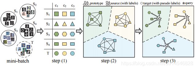
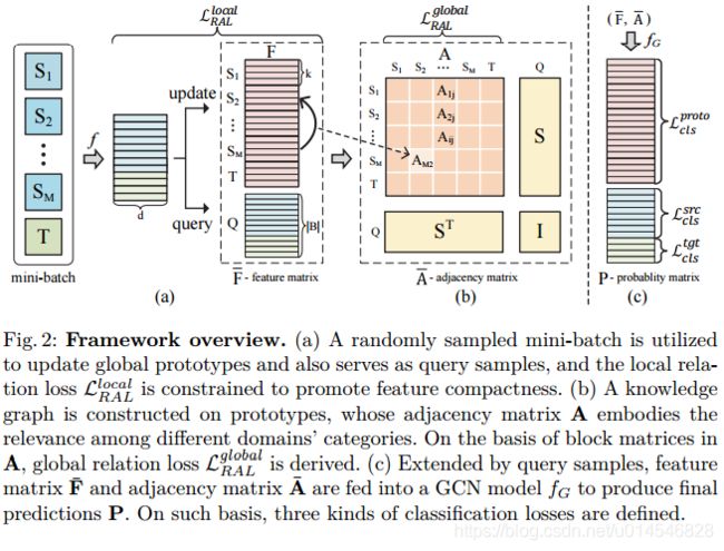
Learning to Combine: Knowledge Aggregation for Multi-Source Domain Adaptation

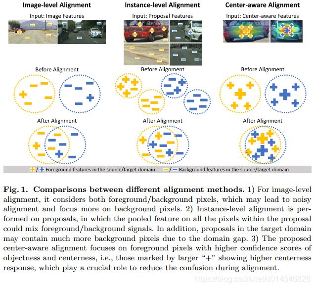
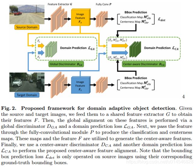
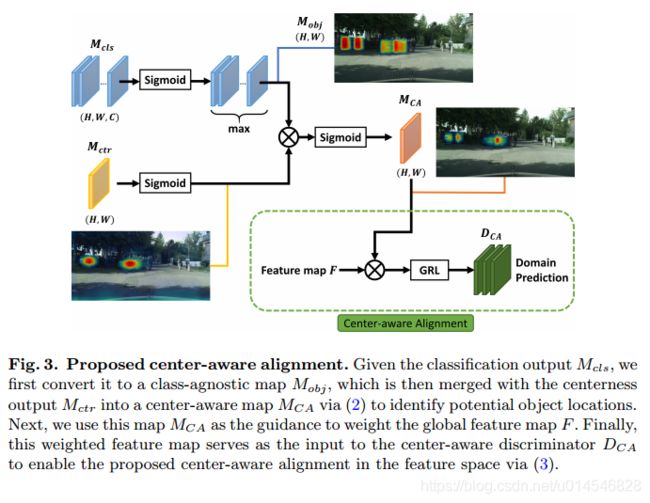
Every Pixel Matters: Center-aware Feature Alignment for Domain Adaptive Object Detector

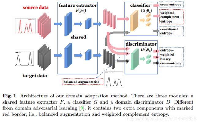
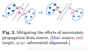
A Balanced and Uncertainty-aware Approach for Partial Domain Adaptation

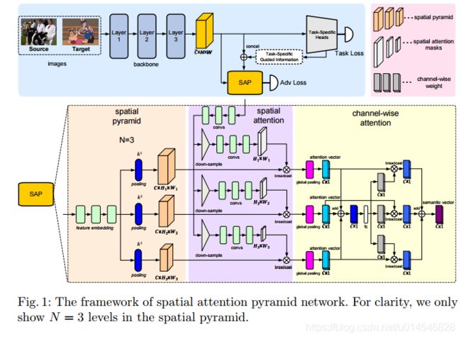
Spatial Attention Pyramid Network for Unsupervised Domain Adaptation

Two-phase Pseudo Label Densification for Self-training based Domain Adaptation

Learning to Detect Open Classes for Universal Domain Adaptation

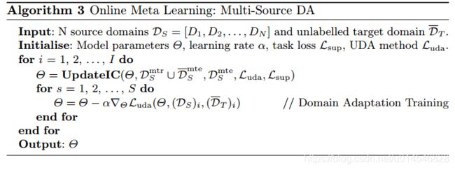
Online Meta-Learning for Multi-Source and Semi-Supervised Domain Adaptation

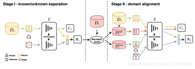
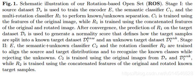
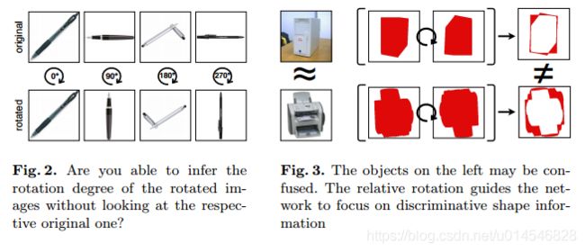
On the Effectiveness of Image Rotation for Open Set Domain Adaptation

HGNet: Hybrid Generative Network for Zero-shot Domain Adaptation

Discriminative Partial Domain Adversarial Network

Dual Mixup Regularized Learning for Adversarial Domain Adaptation

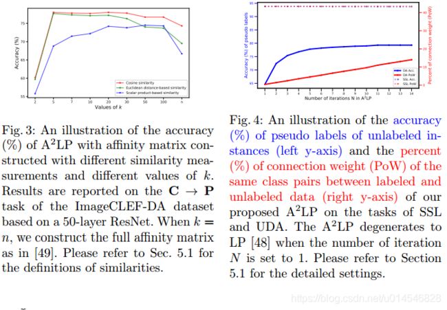
Label Propagation with Augmented Anchors: A Simple Semi-Supervised Learning baseline for Unsupervised Domain Adaptation

Domain2Vec: Domain Embedding for Unsupervised Domain Adaptation

Class-Incremental Domain Adaptation

Progressive Adversarial Networks for Fine-Grained Domain Adaptation

Enhanced Transport Distance for Unsupervised Domain Adaptation

Partial Weight Adaptation for Robust DNN Inference

Rethinking Class-Balanced Methods for Long-Tailed Visual Recognition from a Domain Adaptation Perspective

Unsupervised Domain Adaptation via Structurally Regularized Deep Clustering

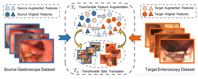
What Can Be Transferred: Unsupervised Domain Adaptation for Endoscopic Lesions Segmentation

Probability Weighted Compact Feature for Domain Adaptive Retrieval

Towards Inheritable Models for Open-Set Domain Adaptation​

Exploring Category-Agnostic Clusters for Open-Set Domain Adaptation

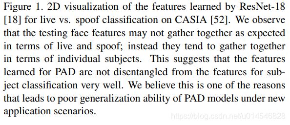
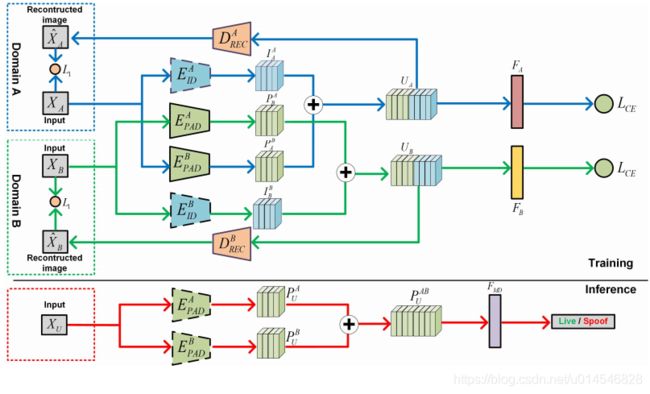
Cross-domain Face Presentation Attack Detection via Multi-domain Disentangled Representation Learning

Unsupervised Domain Adaptation with Hierarchical Gradient Synchronization

Universal Source-Free Domain Adaptation

---

 

[2020 ECCV]

Learning to Combine: Knowledge Aggregation for Multi-Source Domain Adaptation

[paper]

 

Every Pixel Matters: Center-aware Feature Alignment for Domain Adaptive Object Detector

[github] [paper]

 

A Balanced and Uncertainty-aware Approach for Partial Domain Adaptation

[paper]

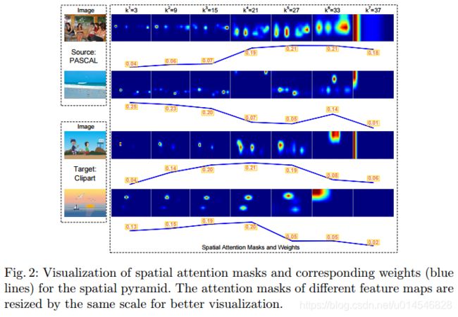
Spatial Attention Pyramid Network for Unsupervised Domain Adaptation

[paper]

 

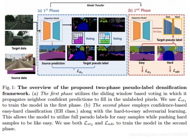
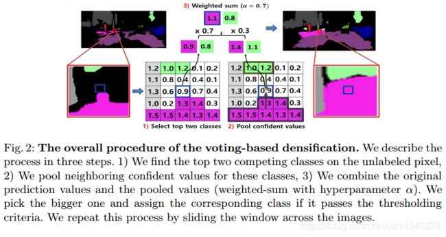
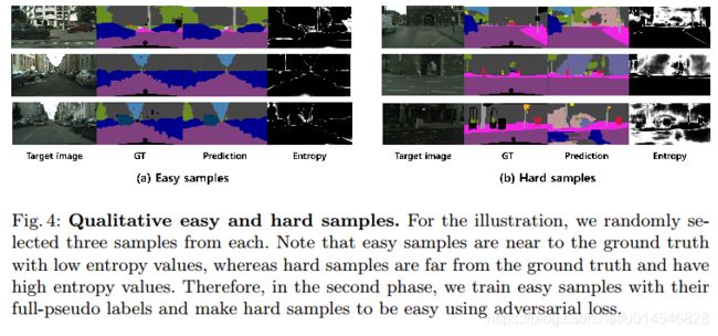
Two-phase Pseudo Label Densification for Self-training based Domain Adaptation

[paper]

 

Learning to Detect Open Classes for Universal Domain Adaptation

[paper]

Fig. 1. (a) The UniDA Setting. There are 3 common, 2 source private and 2 target private classes. The red cross means that the open class “microwave” is easily misclassified to “computer”. (b) Comparison of per-class accuracy and H-score. Assuming that the amount of samples in each category is equal. The classification accuracy of common classes is 80%, and the accuracy of open classes is 50%.

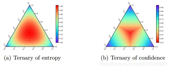
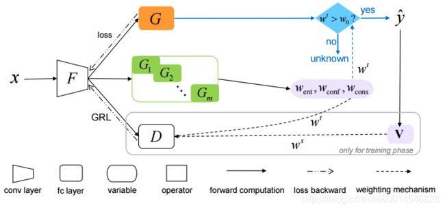
Fig. 2. Heatmap of entropy (a) and confidence (b) w.r.t. the probability values of three classes. Each edge is the value range [0, 1]. The corner area represents class distributions where one label is very likely, while the center area shows nearly uniform distribution.

 

Online Meta-Learning for Multi-Source and Semi-Supervised Domain Adaptation

[paper]

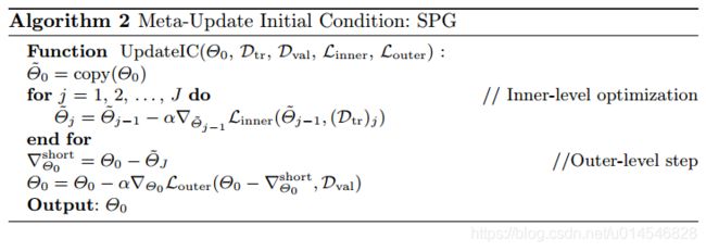
Fig. 1: Left: Exact meta-learning of initial condition with inner loop training DA to convergence is intractable. Right: Online meta-learning alternates between meta-optimization and domain adaptation.

 

 

On the Effectiveness of Image Rotation for Open Set Domain Adaptation

[paper]

 

 

 

HGNet: Hybrid Generative Network for Zero-shot Domain Adaptation

[paper]

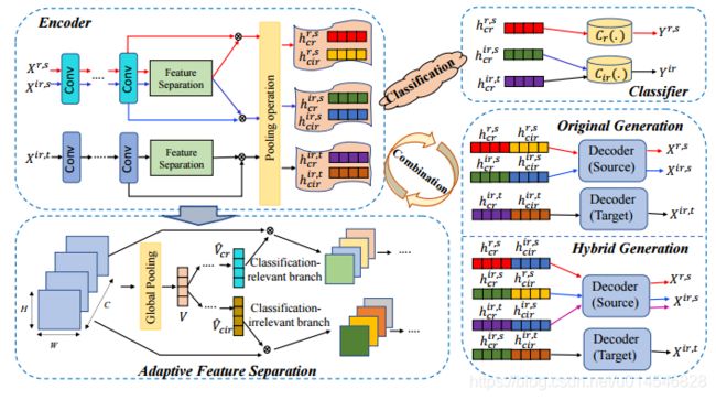
Fig. 1: Overview of the proposed HGNet, which mainly includes four components: encoder, decoder, classifier and adaptive feature separation module. The encoder firstly aims to extract convolutional features, and then the adaptive feature separation module attempts to learn classification-relevant and classificationirrelevant units. On one hand, we utilize label information to guarantee the effect of feature separation. On the other hand, we explore two reconstruction manners to promote the completeness of semantic information and the uniqueness of learned feature.

 

Discriminative Partial Domain Adversarial Network

[paper]

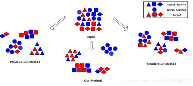
Fig. 1. The main difference of our method against the previous standard domain adaption and partial domain adaption mathods. The blue samples are from source domain and the red ones are from target domain. In standard DA method, source-negative classes can confuse discriminator, leading to performance degeneration. Previous PDA methods can select out most negative classes, but some are still hard to distinguish. Our method not only utilizes hard binary weight narrows the distribution divergence between source-positive and target samples, but also widens the distance between sourcenegative samples and others to reduce negative transfer caused by domain shift.

 

Dual Mixup Regularized Learning for Adversarial Domain Adaptation

[paper]

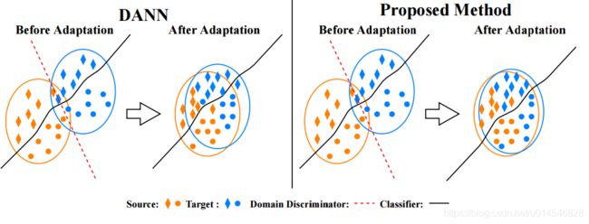
Fig. 1: Comparison of DANN and the proposed method. Left: DANN only tries to match the feature distribution by utilizing adversarial learning; it does not consider the class-aware information in the target domain and samples from the source and target domains may not be sufficient to ensure domain-invariance of the latent space. Right: Our proposed method uses category mixup regularization to enforce prediction consistency in-between samples and domain mixup regularization to explore more intrinsic structures across domains, resulting in better adaptation performance.

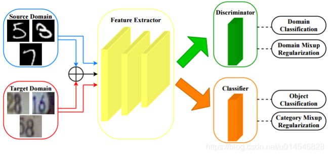
Fig. 2: The architecture of the proposed dual mixup regularized learning (DMRL) method. Our DMRL consists of two mixup-based regularization mechanisms, including category-level mixup regularization and domain-level mixup regularization, which can enhance discriminability and domain-invariance of the latent space. The feature extractor G aims to learn discriminative and domain-invariant features, the domain discriminator D is trained to tell whether the sampled feature comes from the source domain or target domain, and the classifier C is used to conduct object classification.

 

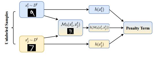
Fig. 3: The framework of unlabeled category mixup regularization.

 

 

Label Propagation with Augmented Anchors: A Simple Semi-Supervised Learning baseline for Unsupervised Domain Adaptation

[paper]

Fig. 1: Visualization of sub-affinity matrices for the settings of (a) SSL, (b) UDA, and (c) UDA with augmented anchors, and their corresponding classification results via the LP. The row-wise and column-wise elements are the unlabeled and labeled instances, respectively. For illustration purposes, we keep elements connecting instances of the same class unchanged, set the others to zero, and sort all instances in the category order using the ground truth category of all data. As we can see, the augmented anchors present better connections with unlabeled target instances compared to the labeled source instances in UDA.

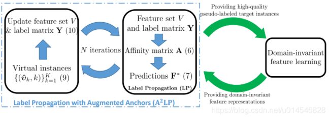
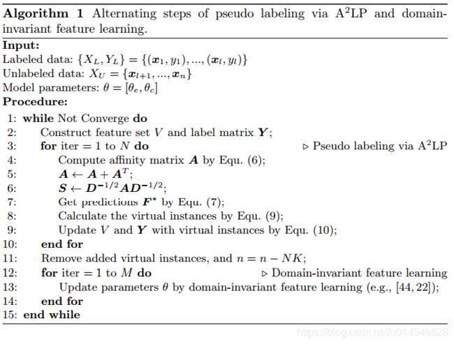
Fig. 2: An illustration of the overall framework of alternating steps of pseudo labeling via A2LP and domain-invariant feature learning. The dashed line rectangle illustrates the algorithm of A2LP, where we iteratively do the steps of (1) augmenting the feature set V and label matrix Y with the generated virtual instances and (2) generating virtual instances by the LP algorithm based on the updated feature set V and label matrix Y .

 

Domain2Vec: Domain Embedding for Unsupervised Domain Adaptation

[paper]

Fig. 1. Our Domain2Vec architecture achieve deep domain embedding by by joint learning of feature disentanglement and Gram matrix. We employ domain disentanglement (red lines) and class disentanglement (blue lines) to extract domain-specific features and category specific features, both trained adversarially. We further apply a mutual information minimizer to enhance the disentanglement.

 

Class-Incremental Domain Adaptation

[paper]

 

 

[2020 CVPR]

Progressive Adversarial Networks for Fine-Grained Domain Adaptation

[paper]

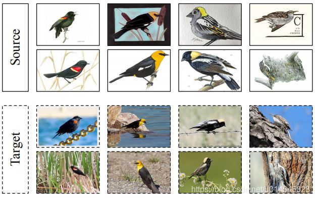
Figure 1. The fine-grained domain adaptation problem is characterized by the entanglement of large inter-domain variations, small inter-class variations, and large intra-class variations, which differs from classic domain adaptation scenario in granularity. From left to right: red-winged blackbirds, yellow-headed blackbirds, bobolinks, and brown creepers.

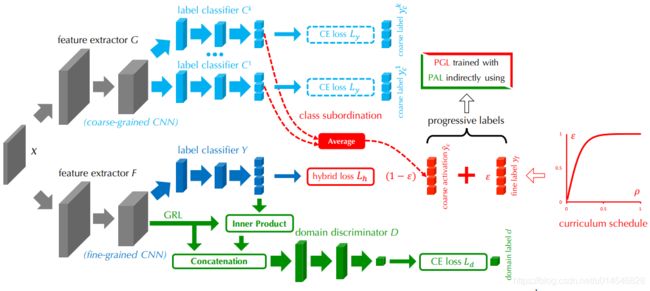
Figure 2. Progressive Adversarial Networks (PAN). A shared feature extractor G and K label predictors C k |k = 1, ..., K together form the coarse-grained CNN (top) for coarse-grained recognition. Similarly, the fine-grained CNN (bottom) contains a feature extractor F and a label predictor Y . Progressive Granularity Learning (PGL, red): the fine-grained ground-truth label yf and the coarse-grained predicted distributions ybc are mixed by ratio ε following a well-established schedule [12] for curriculum learning. We combine the coarse-grained and fine-grained labels into progressive labels via class subordination in label hierarchy (details in Figure 3). Progressive Adversarial Learning (PAL, green): the coarse-to-fine classifier predictions (supervised by progressive labels) are combined with the feature representations by inner product and residual connection, and fed into a domain discriminator D. GRL is the gradient reversal layer [12].

 

Enhanced Transport Distance for Unsupervised Domain Adaptation

[paper]

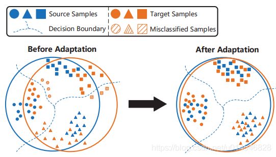
Figure 1. The primary goal of UDA is to generalize the welltrained classifier on the source domain to the unlabeled target domain. Direct application of the learned classifier suffered from the “domain shift” problem, as shown in the left case. UDA methods match the features of different domains, and then reduce the misclassification rate, as shown in the right case.

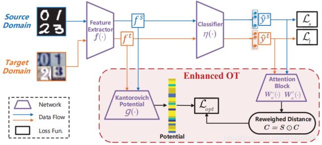
Figure 2. Adaptive model structure diagram for the proposed ETD. The source and target domains share the network weights of the feature extractor. The Kantorovich potential network is constructed by three fully-connected layers, and the attention network is formulated as a single fully connected layer. Blue and Orange arrows represent data flow of the source and target domain respectively. The attention matrix is used to reweigh the optimal transport distance.

 

Partial Weight Adaptation for Robust DNN Inference

[paper]

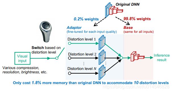
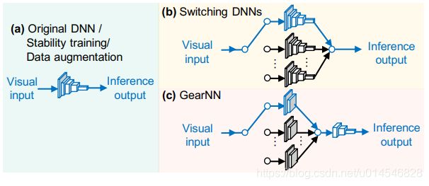
Figure 1: GearNN, an adaptive inference architecture (This is a simplified illustration, DNN layers in the adaptor and those in the base can be interleaved with each other).

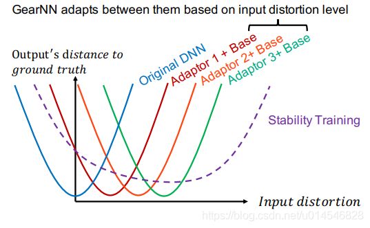
Figure 2: An adaptive DNN can better serve a wide

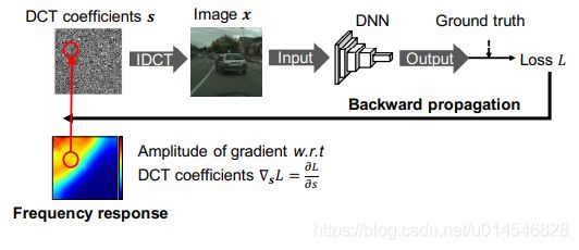
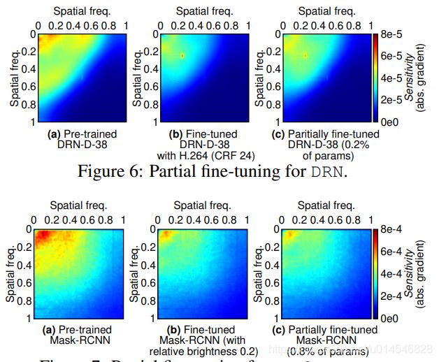
Figure 3: Using the gradient of loss to model the DNN’s freq.-domain perceptual sensitivity (frequency response).

 

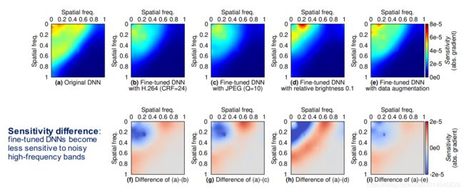
Figure 4: Comparing the DCT spectral sensitivity (frequency response) of the original and fine-tuned DRN-D-38. We use different color palettes for the sensitivity in the 1st row and the sensitivity difference (can be negative) in the 2nd row.

Figure 5: Per-layer average weight value change caused by fine-tuning.

Figure 7: Partial fine-tuning for Mask R-CNN.

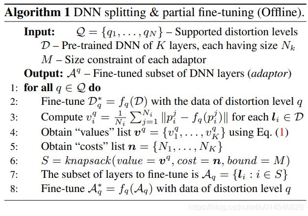
Figure 8: Partial weight fine-tuning workflow.

 

Figure 9: Implementation of GearNN and benchmarks. Modules in blue are active when processing an input instance, while modules in black are overhead.

 

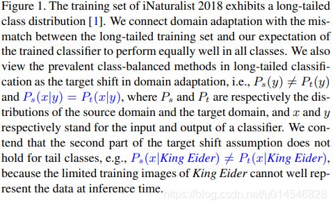
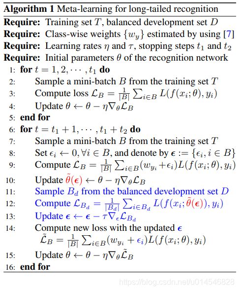
Rethinking Class-Balanced Methods for Long-Tailed Visual Recognition from a Domain Adaptation Perspective

[paper]

 

Unsupervised Domain Adaptation via Structurally Regularized Deep Clustering

[paper]

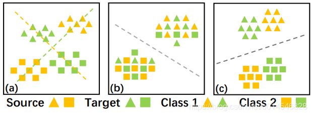
Figure 1. (Best viewed in color.) (a) Illustration of the assumption of structural domain similarity (cf. Section 3). The orange line denotes the classifier trained on the labeled source data and the green one denotes the classifier trained on the labeled target data, i.e. the oracle target classifier. (b) Illustration of damaging intrinsic structures of data discrimination on the target domain by the existing transferring strategy. The dashed line denotes the source classifier adapting to the damaged discrimination of target data, which has a sub-optimal generalization. (c) Illustration of our proposed uncovering strategy. Discriminative target clustering with structural source regularization uncovers intrinsic target discrimination.

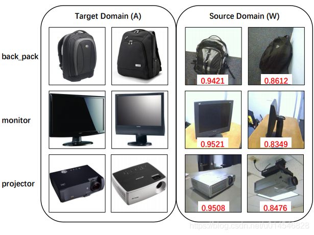
Figure 2. The images on the left are randomly sampled from the target domain A and those on the right are the top-ranked (the 3 rd column) and bottom-ranked (the 4 th column) samples from the source domain W for three classes. Note that the red numbers are the source weights computed by (12).

 

What Can Be Transferred: Unsupervised Domain Adaptation for Endoscopic Lesions Segmentation

[paper]

 

Probability Weighted Compact Feature for Domain Adaptive Retrieval

[paper]

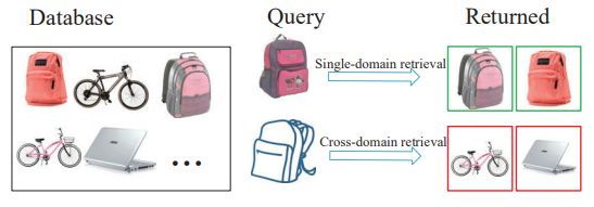
Figure 1. Illustration of our motivation. Many advanced methods have achieved excellent performance in solving the single-domain retrieval problem, but the performance drops significantly when they are used in cross-domain retrieval. In practice, queries and databases usually come from different domains, so it is necessary to solve the problem of cross-domain retrieval.

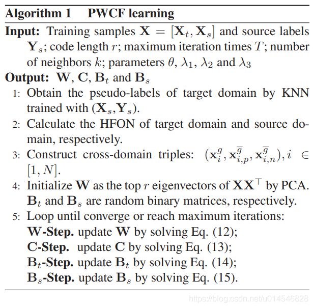
Figure 2. Diagram of PWCF, which includes four parts: 1) BP induced focal-triplet loss, 2) BP induced classification loss, 3) BP induced quantification loss and 4) manifold loss based on Histogram Feature of Neighbors.

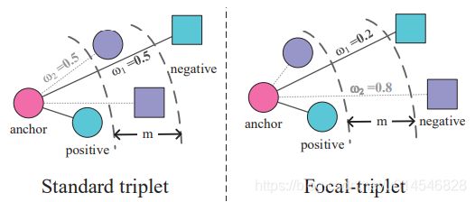
Figure 3. Illustration of the proposed BP induced focal-triplet loss: Standard triplet makes the positive sample closer to the anchor and the negative sample further away from the anchor by the same force (weight). However, positive samples and negative samples may not be separated for hard pairs in this case, which results in training instability. To address it, our BP induced focal-triplet loss can down-weight easy pairs and up-weight hard pairs so as to the distance to the cross-domain positives can be minimized and the distance to the cross-domain negatives can be maximized.

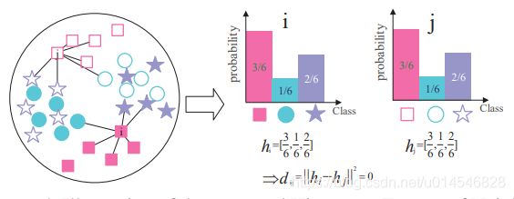
Figure 4. Illustration of the proposed Histogram Feature of Neighbors (HFON): We use different shapes to represent samples of different classes, The samples from the source domain and target domain are represented by solid and hollow shapes, respectively. i and j belong to the same class, but the distance is far. To measure the similarity of cross-domain samples more accurately, we proposed a Histogram Feature of Neighbors according to the neighbor relationship in a domain. For example, we find 6 nearest neighbors of i and j in their respective domains and calculate the probability of each class of these nearest-neighbor samples. HFON vector is made up of these probabilities. Then the HFON distances of similar samples in different domains are close.

 

Towards Inheritable Models for Open-Set Domain Adaptation

[paper]

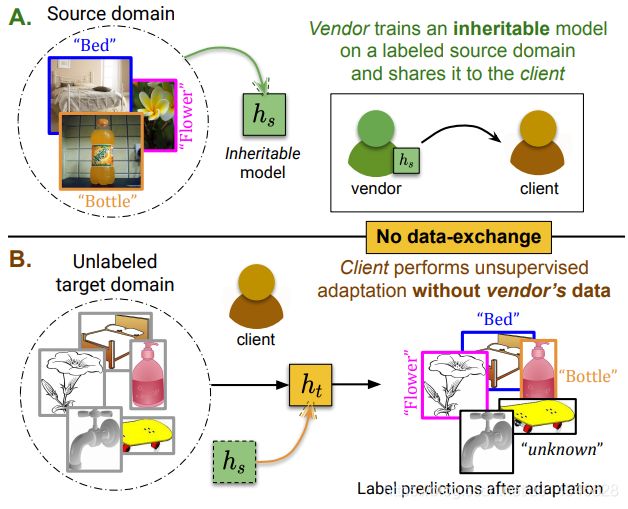
Figure 1. A) We propose inheritable models to transfer the taskspecific knowledge from a model vendor to the client for, B) performing unsupervised open-set domain adaptation in the absence of data-exchange between the vendor and the client.

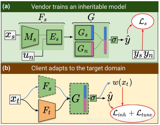
Figure 2. The architectures for A) vendor-side training and B) client-side adaptation. Dashed border denotes a frozen network.

Figure 3. A) An example of a negative instance generated in a 3-dimensional space (d1, d2, d3) using linear interpolation and Featuresplicing. B) Feature-splicing by suppressing the class-discriminative traits (here, we replace the top-(1/3) percentile activation, d1). C) An inheritable model with negative classes. D) Domain-shift before adaptation. E) Successful adaptation. Best viewed in color.

 

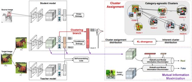
Exploring Category-Agnostic Clusters for Open-Set Domain Adaptation

[paper]

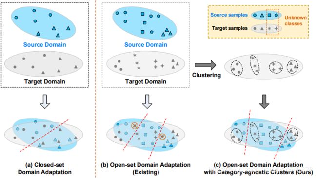
Figure 1. A comparison between (a) closed-set domain adaptation, (b) existing methods for open-set domain adaptation, and (c) our open-set domain adaptation with category-agnostic clusters.

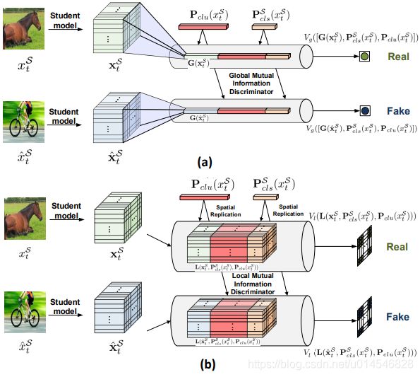
Figure 3. Framework of (a) global mutual information estimation and (b) local mutual information estimation in our SE-C

 

Cross-domain Face Presentation Attack Detection via Multi-domain Disentangled Representation Learning

[paper]

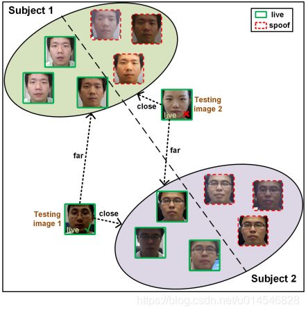
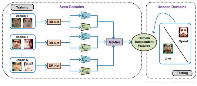
Figure 2. The overview of our approach for cross-domain PAD. Our approach consists of a disentangled representation learning module (DR-Net) and a multi-domain feature learning module (MD-Net). With the face images from different domains as inputs, DR-Net can learn a pair of encoders for disentangled features for PAD and subject classification respectively. The disentangled features are fed to MD-Net to learn domain-independent representations for robust cross-domain PAD.

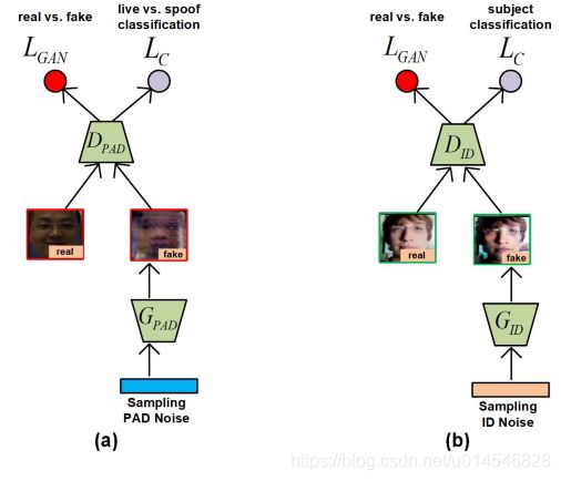
Figure 3. The diagrams of (a) PAD-GAN and (b) ID-GAN in DRNet, which can learn disentangled features for PAD and subject classification, respectively.

 

Unsupervised Domain Adaptation with Hierarchical Gradient Synchronization

[paper]

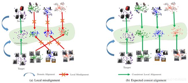
Figure 1. Illustration of (a) local misalignment in methods only with global distribution alignment, and (b) expected alignment on both global domain and local classes. Best viewed in color.

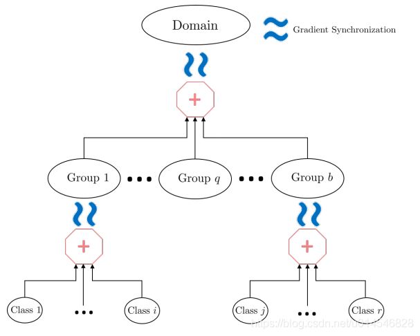
Figure 3. Illustration of the hierarchical distribution alignments and hierarchical gradient synchronization among them

 

Universal Source-Free Domain Adaptation

[paper]

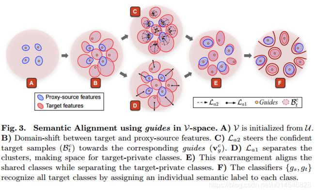
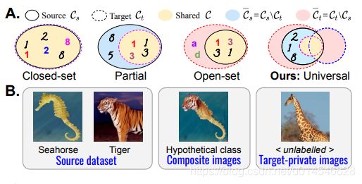
Figure 3: Latent space cluster arrangement during adaptation (see Section 3.1.1).

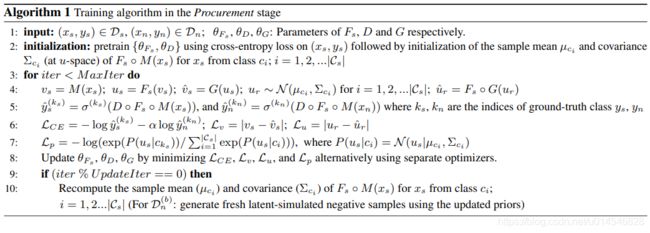
Figure 4: A) Simulated labeled negative samples using randomly created spline segments (in pink), B) Proposed architecture, C) Procurement stage promotes intra-class compactness with inter-class separability.