从零开始搭二维激光SLAM --- 基于ceres的后端优化的代码实现

上一篇文章我们分析了如何使用g2o进行位姿图的优化.

由于g2o天然是进行位姿图优化的, 所以十分契合karto的位姿图的接口, 只需要将对应的顶点和约束分别赋值过去就可以了.

这篇文章我们来看一下另一个比较常用的优化库 Ceres solver.

1 ceres简介

Ceres solver 是谷歌开发的一款用于非线性优化的库, 在激光SLAM和V-SLAM的优化中均有着大量的应用, 如Cartographer, VINS 等等.

ceres的学习可以直接去它的官网上看教程, 谷歌出品的库的文档都很棒. 我在这里就不多说了.
http://ceres-solver.org/tutorial.html

目前网上的很多教程及文章都是翻译的官网, 还是去看第一手资料比较好.

我之前看官方文档的时候做过一个笔记, 感兴趣的同学也可以看看.

ceres笔记
https://blog.csdn.net/tiancailx/article/details/117601117

2 基于ceres的后端优化的代码讲解

接下来就来看一看, 如何使用ceres进行后端优化的求解.

首先是头文件, 头文件基本上一样的, 就是对接口的继承, 就不多说了.

2.1 向位姿图中添加节点

由于ceres不是专门用于位姿图优化的, ceres的本质是求解最小二乘问题.

而目前的slam问题中的位姿图优化的本质都是依赖于最小二乘的, 所以位姿图优化是可以转成最小二乘问题的.

ceres内部没有节点和边的概念, 所以在AddNode函数中, 不像g2o那样可以直接将节点添加到g2o中, 这里首先将节点保存起来, 等到优化的时候再进行计算, 再传入到ceres中.

由于ceres中的数据类型是double, 所以在保存的时候进行了格式的转换.

// 添加节点
void CeresSolver::AddNode(karto::Vertex<karto::LocalizedRangeScan> *pVertex)
{
  karto::Pose2 pose = pVertex->GetObject()->GetCorrectedPose();
  int pose_id = pVertex->GetObject()->GetUniqueId();
  Pose2d pose2d;
  pose2d.x = pose.GetX();
  pose2d.y = pose.GetY();
  pose2d.yaw_radians = pose.GetHeading();
  poses_[pose_id] = pose2d;
}

struct Pose2d
{
  double x;
  double y;
  double yaw_radians;
};

2.2 向位姿图中添加边(约束)

AddConstraint这个函数中的实现和AddNode函数是差不多的.

由于不能直接将边添加到ceres中, 所以在这先做了数据格式的转换, 然后将这个边保存起来.

这里保存的数据分别是 2个节点的 ID, 2个节点间的位姿变换.

在保存位姿的协方差矩阵时进行了求逆的操作, 所以保存的是信息矩阵.

// 添加约束
void CeresSolver::AddConstraint(karto::Edge<karto::LocalizedRangeScan> *pEdge)
{
  karto::LocalizedRangeScan *pSource = pEdge->GetSource()->GetObject();
  karto::LocalizedRangeScan *pTarget = pEdge->GetTarget()->GetObject();
  karto::LinkInfo *pLinkInfo = (karto::LinkInfo *)(pEdge->GetLabel());

  karto::Pose2 diff = pLinkInfo->GetPoseDifference();
  karto::Matrix3 precisionMatrix = pLinkInfo->GetCovariance().Inverse();
  Eigen::Matrix<double, 3, 3> info;
  info(0, 0) = precisionMatrix(0, 0);
  info(0, 1) = info(1, 0) = precisionMatrix(0, 1);
  info(0, 2) = info(2, 0) = precisionMatrix(0, 2);
  info(1, 1) = precisionMatrix(1, 1);
  info(1, 2) = info(2, 1) = precisionMatrix(1, 2);
  info(2, 2) = precisionMatrix(2, 2);
  Eigen::Vector3d measurement(diff.GetX(), diff.GetY(), diff.GetHeading());

  Constraint2d constraint2d;
  constraint2d.id_begin = pSource->GetUniqueId();
  constraint2d.id_end = pTarget->GetUniqueId();
  constraint2d.x = measurement(0);
  constraint2d.y = measurement(1);
  constraint2d.yaw_radians = measurement(2);
  constraint2d.information = info;
  constraints_.push_back(constraint2d);
}

struct Constraint2d
{
  int id_begin;
  int id_end;

  double x;
  double y;
  double yaw_radians;

  Eigen::Matrix3d information;
};

2.3 优化求解

进行求解, 并将优化后的位姿进行保存.

之前都是在保存数据, 真正的计算就在这2个函数里了, 分别是 BuildOptimizationProblem() 与 SolveOptimizationProblem().

// 优化求解
void CeresSolver::Compute()
{
  corrections_.clear();

  ROS_INFO("[ceres] Calling ceres for Optimization");
  ceres::Problem problem;
  BuildOptimizationProblem(constraints_, &poses_, &problem);
  SolveOptimizationProblem(&problem);
  ROS_INFO("[ceres] Optimization finished\n");

  for (std::map<int, Pose2d>::const_iterator pose_iter = poses_.begin(); pose_iter != poses_.end(); ++pose_iter)
  {
    karto::Pose2 pose(pose_iter->second.x, pose_iter->second.y, pose_iter->second.yaw_radians);
    corrections_.push_back(std::make_pair(pose_iter->first, pose));
  }
}

2.4 搭建模型

2.4.1 搭建最小二乘问题

简单解释一下代码.

首先, 通过AngleLocalParameterization::Create()函数定义了角度的更新方式.

这里要注意, 这个 ceres::LocalParameterization *angle_local_parameterization 指针的所有权是 在 problem->SetParameterization() 函数中 交给了 problem 的了, 也就是说, angle_local_parameterization会在problem析构的时候销毁掉.

注意, 这个指针是放在for循环的上边的, 可知, 同一个指针多次传入 AddResidualBlock() 与 SetParameterization() 是可以的. 只是在 problem 析构之后, 这个指针就被销毁了, 不能再使用了.

我在第一次代码写的时候将 angle_local_parameterization 这个指针放在类的成员变量中了, 并只在构造函数中 new 了一次, 当第二次进行优化的时候程序就崩了. 值得注意一下.

之后, 通过 PoseGraph2dErrorTerm::Create() 进行了 CostFunction 的构造.

然后, 将已有的约束信息通过 AddResidualBlock() 添加到优化问题中, 同时, 规定了角度值的更新方式.

最后, 将第一个节点的位姿设置成固定的, 不进行优化和改变.

void CeresSolver::BuildOptimizationProblem(const std::vector<Constraint2d> &constraints, std::map<int, Pose2d> *poses,
                                           ceres::Problem *problem)
{
  if (constraints.empty())
  {
    std::cout << "No constraints, no problem to optimize.";
    return;
  }

  ceres::LocalParameterization *angle_local_parameterization = AngleLocalParameterization::Create();

  for (std::vector<Constraint2d>::const_iterator constraints_iter = constraints.begin();
       constraints_iter != constraints.end(); ++constraints_iter)
  {
    const Constraint2d &constraint = *constraints_iter;
    std::map<int, Pose2d>::iterator pose_begin_iter = poses->find(constraint.id_begin);
    std::map<int, Pose2d>::iterator pose_end_iter = poses->find(constraint.id_end);

    // 对information开根号
    const Eigen::Matrix3d sqrt_information = constraint.information.llt().matrixL();

    // Ceres will take ownership of the pointer.
    ceres::CostFunction *cost_function =
        PoseGraph2dErrorTerm::Create(constraint.x, constraint.y, constraint.yaw_radians, sqrt_information);
    
    problem->AddResidualBlock(cost_function, nullptr,
                              &pose_begin_iter->second.x,
                              &pose_begin_iter->second.y,
                              &pose_begin_iter->second.yaw_radians,
                              &pose_end_iter->second.x,
                              &pose_end_iter->second.y,
                              &pose_end_iter->second.yaw_radians);
    problem->SetParameterization(&pose_begin_iter->second.yaw_radians, angle_local_parameterization);
    problem->SetParameterization(&pose_end_iter->second.yaw_radians, angle_local_parameterization);
  }
  std::map<int, Pose2d>::iterator pose_start_iter = poses->begin();
  problem->SetParameterBlockConstant(&pose_start_iter->second.x);
  problem->SetParameterBlockConstant(&pose_start_iter->second.y);
  problem->SetParameterBlockConstant(&pose_start_iter->second.yaw_radians);
}

2.4.2 角度更新方式

通过重载 () 定义了角度的更新方式, 限定了角度更新后依然处于 [-pi, pi] 之间.代码很简单就不多说了.

之后, 通过 problem->SetParameterization(&pose_begin_iter->second.yaw_radians, angle_local_parameterization); 将这个角度更新方式的限定与角度变量关联起来.

// Defines a local parameterization for updating the angle to be constrained in
// [-pi to pi).
class AngleLocalParameterization
{
public:
  template <typename T>
  bool operator()(const T *theta_radians, const T *delta_theta_radians, T *theta_radians_plus_delta) const
  {
    *theta_radians_plus_delta = NormalizeAngle(*theta_radians + *delta_theta_radians);

    return true;
  }

  static ceres::LocalParameterization *Create()
  {
    return (new ceres::AutoDiffLocalParameterization<AngleLocalParameterization, 1, 1>);
  }
};

// Normalizes the angle in radians between [-pi and pi).
template <typename T>
inline T NormalizeAngle(const T &angle_radians)
{
  // Use ceres::floor because it is specialized for double and Jet types.
  T two_pi(2.0 * M_PI);
  return angle_radians - two_pi * ceres::floor((angle_radians + T(M_PI)) / two_pi);
}

2.4.3 残差的计算

首先通过 PoseGraph2dErrorTerm::Create() 函数进行 ceres::CostFunction 的声明, 并传入 约束的 x, y, theta 以及开方后的信息矩阵 到 PoseGraph2dErrorTerm类的构造函数中将数据进行保存.

之后, 通过重载 () 定义了残差的计算方式. 仿函数的参数就是通过 problem->AddResidualBlock() 传入进来的, 分别是2个位姿的xy与角度.

2个位姿间的残差, 可以这样计算.
构造时传入了这2个位姿间的坐标变换, 而通过这两个节点的位姿又可以算出一个坐标变换, 在正常情况下这2个坐标变换应该是相等的, 所以, 可以让这两个坐标变换的差作为残差.

代码中的 RotationMatrix2D(*yaw_a).transpose() * (p_b - p_a) 就是根据2个节点的位姿算出的坐标变换, p_ab_.cast() 就是传入的这2个位姿间的坐标变换, 通过让2者相减得到 xy的残差.

同理, 角度相减得到角度的残差.

这里, 在计算完成之后, 又将残差左乘了开方后的信息矩阵, 通过协方差矩阵来对计算出的残差添加噪声.

template <typename T>
Eigen::Matrix<T, 2, 2> RotationMatrix2D(T yaw_radians)
{
  const T cos_yaw = ceres::cos(yaw_radians);
  const T sin_yaw = ceres::sin(yaw_radians);

  Eigen::Matrix<T, 2, 2> rotation;
  rotation << cos_yaw, -sin_yaw, sin_yaw, cos_yaw;
  return rotation;
}

// Computes the error term for two poses that have a relative pose measurement
// between them. Let the hat variables be the measurement.
//
// residual =  information^{1/2} * [  r_a^T * (p_b - p_a) - \hat{p_ab}   ]
//                                 [ Normalize(yaw_b - yaw_a - \hat{yaw_ab}) ]
//
// where r_a is the rotation matrix that rotates a vector represented in frame A
// into the global frame, and Normalize(*) ensures the angles are in the range
// [-pi, pi).
class PoseGraph2dErrorTerm
{
public:
  PoseGraph2dErrorTerm(double x_ab, double y_ab, double yaw_ab_radians, const Eigen::Matrix3d &sqrt_information)
      : p_ab_(x_ab, y_ab), yaw_ab_radians_(yaw_ab_radians), sqrt_information_(sqrt_information)
  {
  }

  template <typename T>
  bool operator()(const T *const x_a, const T *const y_a, const T *const yaw_a,
                  const T *const x_b, const T *const y_b, const T *const yaw_b,
                  T *residuals_ptr) const
  {
    const Eigen::Matrix<T, 2, 1> p_a(*x_a, *y_a);
    const Eigen::Matrix<T, 2, 1> p_b(*x_b, *y_b);

    Eigen::Map<Eigen::Matrix<T, 3, 1>> residuals_map(residuals_ptr);

    residuals_map.template head<2>() = RotationMatrix2D(*yaw_a).transpose() * (p_b - p_a) - p_ab_.cast<T>();
    residuals_map(2) = NormalizeAngle((*yaw_b - *yaw_a) - static_cast<T>(yaw_ab_radians_));

    // Scale the residuals by the square root information matrix to account for
    // the measurement uncertainty.
    residuals_map = sqrt_information_.template cast<T>() * residuals_map;

    return true;
  }

  static ceres::CostFunction *Create(double x_ab, double y_ab, double yaw_ab_radians,
                                     const Eigen::Matrix3d &sqrt_information)
  {
    return (new ceres::AutoDiffCostFunction<PoseGraph2dErrorTerm, 3, 1, 1, 1, 1, 1, 1>(
        new PoseGraph2dErrorTerm(x_ab, y_ab, yaw_ab_radians, sqrt_information)));
  }

  EIGEN_MAKE_ALIGNED_OPERATOR_NEW
private:
  // The position of B relative to A in the A frame.
  const Eigen::Vector2d p_ab_;
  // The orientation of frame B relative to frame A.
  const double yaw_ab_radians_;
  // The inverse square root of the measurement covariance matrix.
  const Eigen::Matrix3d sqrt_information_;
};

2.5 进行求解

这块的代码就比较简单了.

首先设置了求解时的参数, 然后调用 ceres::Solve() 进行求解, 并将求解结果的简要报告打印出来.

// Returns true if the solve was successful.
bool CeresSolver::SolveOptimizationProblem(ceres::Problem *problem)
{
  assert(problem != NULL);

  ceres::Solver::Options options;
  options.max_num_iterations = 100;
  options.linear_solver_type = ceres::SPARSE_NORMAL_CHOLESKY;

  ceres::Solver::Summary summary;
  ceres::Solve(options, problem, &summary);

  std::cout << summary.BriefReport() << '\n';
  return summary.IsSolutionUsable();
}

3 运行

3.1 依赖

这篇文章的代码是需要依赖 1.13.0 版本的ceres库, 如果没装ceres的需要先安装一下.
我将ceres库的安装包放在了 工程Creating-2D-laser-slam-from-scratch/TrirdParty文件加内, 可以直接解压安装.

安装的方法可以看一下 install_dependence.sh 脚本中的安装指令, 也可以直接执行这个脚本进行所有依赖项的安装.

安装完了ceres之后, 编译代码, 如果一切顺利的话是可以编译通过的.

这里要说一下, 很多同学说代码在ubuntu 18 或者其他的ubuntu版本上编译不过, 这我也没啥办法, 我一直用的是 1604, 没试过其他的版本. 如果实在编译不过就看看文章吧, 或者看看源码.

3.2 运行

本篇文章对应的数据包, 请在我的公众号中回复 lesson6 获得，并将launch中的bag_filename更改成您实际的目录名。

我将之前使用过的数据包的链接都放在腾讯文档里了, 腾讯文档的地址如下:
https://docs.qq.com/sheet/DVElRQVNlY0tHU01I?tab=BB08J2

通过如下命令运行本篇文章对应的程序
roslaunch lesson6 karto_slam_outdoor.launch solver_type:=ceres_solver

3.3 结果分析

启动之后, 会显示出使用的优化器的具体类型.

[ INFO] [1637029966.740001825]: ----> Karto SLAM started.
[ INFO] [1637029966.790614727]: Use back end.
[ INFO] [1637029966.790716666]: solver type is CeresSolver.

在运行前期, 由于没有找到回环, 所以一直没有进行优化. 在最后阶段产生回环时, 会调用基于ceres的优化, 并打印处如下的log.

[ INFO] [1637030162.060933669, 1606808844.440984444]: [ceres] Calling ceres for Optimization
Ceres Solver Report: Iterations: 8, Initial cost: 4.364248e-02, Final cost: 7.465524e-15, Termination: CONVERGENCE
[ INFO] [1637030162.089423589, 1606808844.471175613]: [ceres] Optimization finished

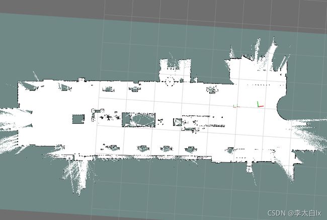
可以看到, 优化前的cost是 e-02 量级的, 优化后的cost是 e-15 量级的, 效果十分明显.

优化前

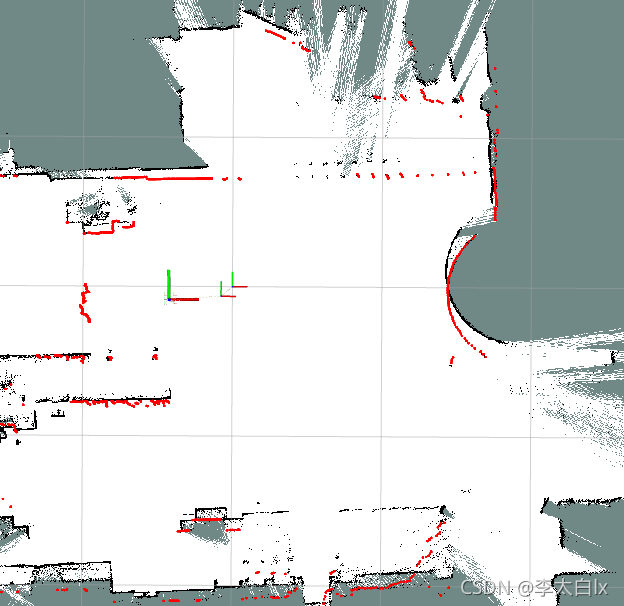
优化后

最终的地图

最终的cost

看一下最终的cost, 可以看到, 之前优化后的cost都是 e-15 这种级别的, 但是最后一次的cost是 e-02, 变大了很多. 原因还不清楚.

猜测可能是由于数据数据突然结束了, 导致其实还存在优化的空间???

有了解的同学可以评论告诉我一下, 十分感谢.

[ INFO] [1637032488.825845405, 1606808848.018522836]: [ceres] Calling ceres for Optimization
Ceres Solver Report: Iterations: 8, Initial cost: 6.562447e-02, Final cost: 5.582333e-15, Termination: CONVERGENCE
[ INFO] [1637032488.850353017, 1606808848.038643242]: [ceres] Optimization finished

[ INFO] [1637032489.159521180, 1606808848.351362847]: [ceres] Calling ceres for Optimization
Ceres Solver Report: Iterations: 8, Initial cost: 2.219165e-02, Final cost: 6.116063e-15, Termination: CONVERGENCE
[ INFO] [1637032489.183078270, 1606808848.371497779]: [ceres] Optimization finished

[ INFO] [1637032489.493828053, 1606808848.683609037]: [ceres] Calling ceres for Optimization
Ceres Solver Report: Iterations: 9, Initial cost: 4.919947e+01, Final cost: 1.920770e-02, Termination: CONVERGENCE
[ INFO] [1637032489.519517167, 1606808848.703747883]: [ceres] Optimization finished

4 总结

通过这篇文章, 我们知道了如何使用ceres进行后端优化问题的搭建与计算, 并体验了优化前后的地图效果与cost值.

下篇文章将使用gtsam来进行后端优化的计算.