学习日记1
目录
Goolge Colab学习
colab简单教程
stackoverflow
卷积神经网络
深度学习迭代次数
python (),[], {}
pd.DataFrame()函数解析(最清晰的解释)
欧式距离 马氏距离
深度学习 模型训练超参数调整
rnn学习
损失和准确性
matplotlib绘制堆叠柱状图
Goolge Colab学习
前提,要科学上网 = =
优点:免费使用GPU进行计算
Colab简介:https://colab.research.google.com/notebooks/welcome.ipynb
谷歌硬盘和colab是分开的,需要把硬盘挂载到colab上面
操作目的:在colab中可以直接读写google drive的目录,模型可以直接保存在drive上,很方便
操作过程
#挂载谷歌硬盘,不需要重复执行
from google.colab import drive
drive.mount('/content/drive')
运行后出现下图,点链接复制验证码

点击蓝色链接,进入下图,选择谷歌邮箱点击

点击允许授予权限,跳出验证码后复制到输入框中后敲回车Enter
![]()
左侧如下显示

这一段代码也可以不写,按下图操作挂载谷歌硬盘,就可以直接%cd切换目录

测试GPU
%tensorflow_version 2.x   testing the GPU
import tensorflow as tf
device_name = tf.test.gpu_device_name()
if device_name != '/device:GPU:0':
  raise SystemError('GPU device not found')
print('Found GPU at: {}'.format(device_name))
!/opt/bin/nvidia-smi #查看显卡信息
如何让google colab不断连
https://blog.csdn.net/liupeng19970119/article/details/105625334
1.crtl+shift+i进入网页代码
2.在上图的红线地方输入下面代码后确定:

function ClickConnect(){
  colab.config
  console.log("Connnect Clicked - Start");
  document.querySelector("#top-toolbar > colab-connect-button").shadowRoot.querySelector("#connect").click();
  console.log("Connnect Clicked - End");
};
setInterval(ClickConnect, 60000)
3.输入完成之后得到上面红线效果,每隔60秒会点击一次。
另一个代码
function ClickConnect(){
console.log("Working");
document.querySelector("colab-toolbar-button#connect").click()
}
var id=setInterval(ClickConnect,5*60000)   //5分钟点一次,改变频率把5换成其他数即可,单位分钟
//要提前停止,请输入运行以下代码:    clearInterval(id)
https://blog.csdn.net/weixin_44754037/article/details/123356730
colab简单教程
来源:
https://towardsdatascience.com/image-classification-in-10-minutes-with-mnist-dataset-54c35b77a38d
Downloading the MNIST Dataset
The MNIST dataset is one of the most common datasets used for image classification and accessible from many different sources. In fact, even Tensorflow and Keras allow us to import and download the MNIST dataset directly from their API. Therefore, I will start with the following two lines to import TensorFlow and MNIST dataset under the Keras API.
import tensorflow as tf
(x_train, y_train), (x_test, y_test) = tf.keras.datasets.mnist.load_data()
To visualize these numbers, we can get help from matplotlib.
import matplotlib.pyplot as plt
%matplotlib inline # Only use this if using iPython
image_index = 7777 # You may select anything up to 60,000
print(y_train[image_index]) # The label is 8
plt.imshow(x_train[image_index], cmap='Greys')
When we run the code above, we will get the greyscale visualization of the RGB codes as shown below.

A visualization of the sample image at index 7777
We also need to know the shape of the dataset to channel it to the convolutional neural network. Therefore, I will use the “shape” attribute of NumPy array with the following code:
x_train.shapeReshaping and Normalizing the Images
# Reshaping the array to 4-dims so that it can work with the Keras API
x_train = x_train.reshape(x_train.shape[0], 28, 28, 1)
x_test = x_test.reshape(x_test.shape[0], 28, 28, 1)
input_shape = (28, 28, 1)
# Making sure that the values are float so that we can get decimal points after division
x_train = x_train.astype('float32')
x_test = x_test.astype('float32')
# Normalizing the RGB codes by dividing it to the max RGB value.
x_train /= 255
x_test /= 255
print('x_train shape:', x_train.shape)
print('Number of images in x_train', x_train.shape[0])
print('Number of images in x_test', x_test.shape[0])
Building the Convolutional Neural Network
We will build our model by using high-level Keras API which uses either TensorFlow or Theano on the backend. I would like to mention that there are several high-level TensorFlow APIs such as Layers, Keras, and Estimators which helps us create neural networks with high-level knowledge. However, this may lead to confusion since they all vary in their implementation structure. Therefore, if you see completely different codes for the same neural network although they all use TensorFlow, this is why. I will use the most straightforward API which is Keras. Therefore, I will import the Sequential Model from Keras and add Conv2D, MaxPooling, Flatten, Dropout, and Dense layers. I have already talked about Conv2D, Maxpooling, and Dense layers. In addition, Dropout layers fight with the overfitting by disregarding some of the neurons while training while Flatten layers flatten 2D arrays to 1D arrays before building the fully connected layers.
# Importing the required Keras modules containing model and layers
from tensorflow.keras.models import Sequential
from tensorflow.keras.layers import Dense, Conv2D, Dropout, Flatten, MaxPooling2D
# Creating a Sequential Model and adding the layers
model = Sequential()
model.add(Conv2D(28, kernel_size=(3,3), input_shape=input_shape))
model.add(MaxPooling2D(pool_size=(2, 2)))
model.add(Flatten()) # Flattening the 2D arrays for fully connected layers
model.add(Dense(128, activation=tf.nn.relu))
model.add(Dropout(0.2))
model.add(Dense(10,activation=tf.nn.softmax))
Compiling and Fitting the Model
model.compile(optimizer='adam',
              loss='sparse_categorical_crossentropy',
              metrics=['accuracy'])
model.fit(x=x_train,y=y_train, epochs=10)
Evaluating the Model
model.evaluate(x_test, y_test)We achieved 98.5% accuracy with such a basic model. To be frank, in many image classification cases (e.g. for autonomous cars), we cannot even tolerate 0.1% error since, as an analogy, it will cause 1 accident in 1000 cases. However, for our first model, I would say the result is still pretty good. We can also make individual predictions with the following code:
image_index = 4444
plt.imshow(x_test[image_index].reshape(28, 28),cmap='Greys')
pred = model.predict(x_test[image_index].reshape(1, 28, 28, 1))
print(pred.argmax())
Congratulations!
You have successfully built a convolutional neural network to classify handwritten digits with Tensorflow’s Keras API. You have achieved accuracy of over 98% and now you can even save this model & create a digit-classifier app! If you are curious about saving your model, I would like to direct you to the Keras Documentation. After all, to be able to efficiently use an API, one must learn how to read and use the documentation.
stackoverflow
https://stackoverflow.com/ csdn找不到可以去这查
卷积神经网络
https://www.bilibili.com/video/BV1fE411k77X/?spm_id_from=333.788.videocard.0

https://brohrer.mcknote.com/zh-Hans/how_machine_learning_works/how_convolutional_neural_networks_work.html
我们的圈和叉例子和图像辨识有关,不过 CNN 也能处理其他型态的数据,技巧是将任何数据转成类似图片的形式。例如,我们可以将音频根据时间细分,再将每一小段的声音分成低音、中音、高音或其他更高的频率。如此一来,我们就可以把这些信息组成一个二维矩阵,其中各行代表不同时间、各列代表不同频率。在这张假图片里,越相近的「像素」,彼此之间的关联性越高。CNN 很擅长处理这样的数据,研究者们也发挥创意,将自然语言处理(natural language processing)中的文本数据、和新药研发过程中的化学数据都转成 CNN 可以处理的形式。
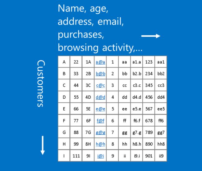
不过当每一横列(row)代表一位顾客、每一直行(column)分别代表这位顾客的姓名、信箱、购买和浏览纪录等不同信息时,这种顾客数据并非 CNN 可以处理的形式。因为在这个例子里,行和列的位置并不重要,也就是说在不影响信息的情况下,它们可以被任意排列。相较之下,一张图片里像素的行列位置如果被调换,通常会丧失原本的意义。
所以使用 CNN 的一个诀窍是如果数据不会受改变行列顺序所影响,这种数据就不适合使用 CNN 处理。不过如果可以将问题转成类似图片辨识的形式,那 CNN 很可能是最理想的工具。
深度学习迭代次数
https://zhuanlan.zhihu.com/p/195368815
01 当loss值收敛时结束迭代
02 使用验证集来检验训练成果
autoencoder.fit(train_data, train_data,
epochs=50,
batch_size=128,
shuffle=True,
validation_data=(noisy_imgs, data_test)
)
python (),[], {}
https://blog.csdn.net/yy_lemon/article/details/109211639
1、python ()表示元祖,元祖是一种不可变序列
1)创建如:tuple = (1,2,3) 取数据 tuple[0]...... tuple[0,2].....tuple[1,2]......
2 ) 修改元祖:元祖是不可修改的
3)删除元祖 del tuple
4)内置函数:
cmp(tuple1,tuple2):比较两个元祖
len(tuple):计算元祖的长度
max(tuple):最大值
min(tuple):最小值
tuple(seq):将列表转为元祖
2、python []表示列表,列表是可变的序列
1)创建列表l = [1,2,3,4]取数据l[0]........
2)列表可修改
3)内置函数
cmp(list1,list2):比较两个元祖
len(list):计算元祖的长度
max(list):最大值
min(list):最小值
list(seq):将元祖转为列表
list.append(obj):在列表末尾新增对象
list.pop():移除某个数据
list.remove:移除某个列表中匹配的第一个值
list.sort():排序
list.reverse():反转列表
list.count(bj):计算对象在列表中出现的次数
list.insert(index,obj) :在某个位置插入对象
3、python {} 字典;字典是可变的容器,使用比较灵活
1)创建字典:dict = {"a":1,"b":2}. 字典是一对:key, value的键值对 取数据dict['a'],
2)可修改
3)删除:del dict["a"] 删除某对数据 del dict 删除字典 dict.clear()清除字典所有条目
4)内置函数
cmp(dict1,dict2):比较两个元祖
len(dict):计算元祖的长度
dict.clear():删除字典数据
dict.get(key, default=None):返回指定值,如果没有返回指定默认值
dict.has_key(key):判断值是否存在,返回true,false
dict.item()以列表值返回返回可遍历的(键,值)的元祖
dict.key()返回字典所有的key值
Classification via Decision Trees in WEKA
weka分类教程,可惜文件下载不了
https://www.cnblogs.com/zlslch/p/6844482.html
weka基础教程,有TP、FP、recall等的解释
原文链接:https://blog.csdn.net/tefuirnever/article/details/93708964
pd.DataFrame()函数解析(最清晰的解释)
DataFrame是Python中Pandas库中的一种数据结构,它类似excel,是一种二维表。
文章目录
0 简介
1 创建DataFrame
1.1 使用numpy函数创建
1.2 直接创建
1.3 使用字典创建
2 DataFrame属性
2.1 查看列的数据类型
2.2 查看DataFrame的头尾
2.3 查看行名与列名
2.4 查看数据值
2.5 查看行列数
2.6 切片
2.7 索引
3 DataFrame操作
3.1 转置
3.2 描述性统计
3.3 计算
3.4 新增
3.5 合并
3.6 去重
参考文章
0 简介
DataFrame的单元格可以存放数值、字符串等,这和excel表很像,同时DataFrame可以设置列名columns与行名index。
1 创建DataFrame
以下的实验是在python3.5.6版本下进行的。先导入所需库
import pandas as pd
import numpy as np
#pandas常与numpy一起配合使用
1.1 使用numpy函数创建
可以直接通过pandas的DataFrame函数进行创建。
df1 = pd.DataFrame(np.random.randn(3, 3), index=list('abc'), columns=list('ABC'))
print(df1)
'''
运行结果
           A         B         C
 a -0.612978  0.237191  0.312969
 b -1.281485  1.135944  0.162456
 c  2.232905  0.200209  0.028671
'''
其中第一个参数是存放在DataFrame里的数据,第二个参数index设置行名,第三个参数columns设置列名。
其中后两个参数可以使用list输入,list的长度要和DataFrame的大小匹配,不然会报错。
当然,这两个参数是可选的,你可以选择不设置,而且这两个list是可以一样的。
1.2 直接创建
df4 = pd.DataFrame([[1, 2, 3],
                    [2, 3, 4],
                    [3, 4, 5]],
                   index=list('abc'), columns=list('ABC'))
print(df4)
'''
运行结果
    A  B  C
 a  1  2  3
 b  2  3  4
 c  3  4  5
'''
1.3 使用字典创建
dic1 = {
'name': [
'张三', '李四', '王二麻子', '小淘气'], 'age': [
37, 30, 50, 16], 'gender': [
'男', '男', '男', '女']}
df5 = pd.DataFrame(dic1)
print(df5)
# age gender name
# 0 37 男 张三
# 1 30 男 李四
# 2 50 男 王二麻子
# 3 16 女 小淘气
2 DataFrame属性
2.1 查看列的数据类型
print(df5.dtypes)
# age int64
# gender object
# name object
# dtype: object
2.2 查看DataFrame的头尾
使用head可以查看前几行的数据,默认的是前5行,不过也可以自己设置。
使用tail可以查看后几行的数据,默认也是5行,参数可以自己设置。
比如看前5行。
df6 = pd.DataFrame(np.arange(36).reshape(6, 6), index=list('abcdef'), columns=list('ABCDEF'))
print(df6)
# A B C D E F
# a 0 1 2 3 4 5
# b 6 7 8 9 10 11
# c 12 13 14 15 16 17
# d 18 19 20 21 22 23
# e 24 25 26 27 28 29
# f 30 31 32 33 34 35
print(df6.head())
# A B C D E F
# a 0 1 2 3 4 5
# b 6 7 8 9 10 11
# c 12 13 14 15 16 17
# d 18 19 20 21 22 23
# e 24 25 26 27 28 29
比如只看前2行。
print(df6.head(2))
# A B C D E F
# a 0 1 2 3 4 5
# b 6 7 8 9 10 11
比如看后5行。
print(df6.tail())
# A B C D E F
# b 6 7 8 9 10 11
# c 12 13 14 15 16 17
# d 18 19 20 21 22 23
# e 24 25 26 27 28 29
# f 30 31 32 33 34 35
比如只看后2行。
print(df6.tail(2))
# A B C D E F
# e 24 25 26 27 28 29
# f 30 31 32 33 34 35
2.3 查看行名与列名
使用index查看行名,columns查看列名。
print(df6.index)
print(df6.columns)
# Index(['a', 'b', 'c', 'd', 'e', 'f'], dtype='object')
# Index(['A', 'B', 'C', 'D', 'E', 'F'], dtype='object')
2.4 查看数据值
使用values可以查看DataFrame里的数据值,返回的是一个数组。
print(df6.values)
# [[ 0 1 2 3 4 5]
# [ 6 7 8 9 10 11]
# [12 13 14 15 16 17]
# [18 19 20 21 22 23]
# [24 25 26 27 28 29]
# [30 31 32 33 34 35]]
比如说查看某一列所有的数据值。
print(df6['B'].values)
[ 1 7 13 19 25 31]
如果查看某一行所有的数据值。使用iloc查看数据值(但是好像只能根据行来查看?),iloc是根据数字索引(也就是行号)。可以看一下博客pandas.iloc()函数解析。
print(df6.iloc[0])
# A 0
# B 1
# C 2
# D 3
# E 4
# F 5
# Name: a, dtype: int32
2.5 查看行列数
使用shape查看行列数,参数为0表示查看行数,参数为1表示查看列数。
print(df6.shape[0])
print(df6.shape[1])
# 6
# 6
2.6 切片
使用冒号进行切片。
print(df6['a':'b'])
# A B C D E F
# a 0 1 2 3 4 5
# b 6 7 8 9 10 11
2.7 索引
print(df6.loc[:,'A':'B'])
# A B
# a 0 1
# b 6 7
# c 12 13
# d 18 19
# e 24 25
# f 30 31
切片表示的是行切片
索引表示的是列索引
3 DataFrame操作
3.1 转置
直接字母T,线性代数上线。
print(df6.T)
# a b c d e f
# A 0 6 12 18 24 30
# B 1 7 13 19 25 31
# C 2 8 14 20 26 32
# D 3 9 15 21 27 33
# E 4 10 16 22 28 34
# F 5 11 17 23 29 35
3.2 描述性统计
使用describe可以对数据根据列进行描述性统计。
print(df6.describe())
# A B C D E F
# count 6.000000 6.000000 6.000000 6.000000 6.000000 6.000000
# mean 15.000000 16.000000 17.000000 18.000000 19.000000 20.000000
# std 11.224972 11.224972 11.224972 11.224972 11.224972 11.224972
# min 0.000000 1.000000 2.000000 3.000000 4.000000 5.000000
# 25% 7.500000 8.500000 9.500000 10.500000 11.500000 12.500000
# 50% 15.000000 16.000000 17.000000 18.000000 19.000000 20.000000
# 75% 22.500000 23.500000 24.500000 25.500000 26.500000 27.500000
# max 30.000000 31.000000 32.000000 33.000000 34.000000 35.000000
如果有的列是非数值型的,那么就不会进行统计。
如果想对行进行描述性统计,转置后再进行describe。
3.3 计算
使用sum默认对每列求和,sum(1)为对每行求和。
print(df6.sum())
# A 90
# B 96
# C 102
# D 108
# E 114
# F 120
# dtype: int64
print(df6.sum(1))
# a 15
# b 51
# c 87
# d 123
# e 159
# f 195
# dtype: int64
数乘运算使用apply。
print(df6.apply(lambda x: x * 2))
# A B C D E F
# a 0 2 4 6 8 10
# b 12 14 16 18 20 22
# c 24 26 28 30 32 34
# d 36 38 40 42 44 46
# e 48 50 52 54 56 58
# f 60 62 64 66 68 70
乘方运算跟matlab类似,直接使用两个*。
print(df6**2)
# A B C D E F
# a 0 1 4 9 16 25
# b 36 49 64 81 100 121
# c 144 169 196 225 256 289
# d 324 361 400 441 484 529
# e 576 625 676 729 784 841
# f 900 961 1024 1089 1156 1225
3.4 新增
扩充列可以直接像字典一样,列名对应一个list,但是注意list的长度要跟index的长度一致。
df6['G']=['999','999','999','999','999','999']
print(df6)
# A B C D E F G
# a 0 1 2 3 4 5 999
# b 6 7 8 9 10 11 999
# c 12 13 14 15 16 17 999
# d 18 19 20 21 22 23 999
# e 24 25 26 27 28 29 999
# f 30 31 32 33 34 35 999
还可以使用insert,使用这个方法可以指定把列插入到第几列,其他的列顺延。
df6.insert(0, 'QQ', ['999','999','999','999','999','999'])
print(df6)
# QQ A B C D E F
# a 999 0 1 2 3 4 5
# b 999 6 7 8 9 10 11
# c 999 12 13 14 15 16 17
# d 999 18 19 20 21 22 23
# e 999 24 25 26 27 28 29
# f 999 30 31 32 33 34 35
3.5 合并
使用join可以将两个DataFrame合并,但只根据行列名合并,并且以作用的那个DataFrame的为基准。
# 也就是以df6为基准。
df7 = pd.DataFrame(['my', 'name', 'is', 'a', 'b', 'c'], index=list('abcdef'), columns=list('G'))
df8 = df6.join(df7)
print(df8)
# A B C D E F G
# a 0 1 2 3 4 5 my
# b 6 7 8 9 10 11 name
# c 12 13 14 15 16 17 is
# d 18 19 20 21 22 23 a
# e 24 25 26 27 28 29 b
# f 30 31 32 33 34 35 c
但是,join这个方法还有how这个参数可以设置,合并两个DataFrame的交集或并集。参数为’inner’表示交集,'outer’表示并集。
df7 = pd.DataFrame(['2', '6', '7', '19', '44', '77'], index=list('abekld'), columns=list('G'))
df8=df6.join(df7,how='inner')
df9=df6.join(df7,how='outer')
print(df8)
# A B C D E F G
# a 0 1 2 3 4 5 2
# b 6 7 8 9 10 11 6
# d 18 19 20 21 22 23 77
# e 24 25 26 27 28 29 7
print(df9)
# A B C D E F G
# a 0.0 1.0 2.0 3.0 4.0 5.0 2
# b 6.0 7.0 8.0 9.0 10.0 11.0 6
# c 12.0 13.0 14.0 15.0 16.0 17.0 NaN
# d 18.0 19.0 20.0 21.0 22.0 23.0 77
# e 24.0 25.0 26.0 27.0 28.0 29.0 7
# f 30.0 31.0 32.0 33.0 34.0 35.0 NaN
# k NaN NaN NaN NaN NaN NaN 19
# l NaN NaN NaN NaN NaN NaN 44
如果要合并多个Dataframe,可以用list把几个Dataframe装起来,然后使用concat转化为一个新的Dataframe。
df10 = pd.DataFrame([1, 2, 3, 4, 5, 6],
index=list('ABCDEF'), columns=['a'])
df11 = pd.DataFrame([10, 20, 30, 40, 50, 60],
index=list('ABCDEF'), columns=['b'])
df12 = pd.DataFrame([100, 200, 300, 400, 500, 600],
index=list('ABCDEF'), columns=['c'])
list1 = [df10.T, df11.T, df12.T]
df13 = pd.concat(list1)
print(df13)
# A B C D E F
# a 1 2 3 4 5 6
# b 10 20 30 40 50 60
# c 100 200 300 400 500 600
3.6 去重
df.drop_duplicates(subset=None,
keep='first',
inplace=False
)
参数:
subset:指定是哪些列重复。
keep:去重后留下第几行,{‘first’, ‘last’, False}, default ‘first’},如果是False,则去除全部重复的行。
inplace:是否作用于原来的df。
df14 = pd.DataFrame(data=[[1, 2, 3],
[1, 2, 4],
[1, 2, 4],
[1, 2, 3],
[1, 2, 5],
[1, 2, 5]],
index=list('ABCDEF'),
columns=['a', 'b', 'c'])
print(df14)
# a b c
# A 1 2 3
# B 1 2 4
# C 1 2 4
# D 1 2 3
# E 1 2 5
# F 1 2 5
去除重复行,保留重复行中最后一行
df14.drop_duplicates(keep='last')
# a b c
# C 1 2 4
# D 1 2 3
# F 1 2 5
去除’c’列中有重复的值所在的行
print(df14.drop_duplicates(subset=('c',)))
# a b c
# A 1 2 3
# B 1 2 4
# E 1 2 5
欧式距离 马氏距离
欧氏距离定义: 欧氏距离( Euclidean distance)是一个通常采用的距离定义,它是在m维空间中两个点之间的真实距离。
在二维和三维空间中的欧式距离的就是两点之间的距离,二维的公式是
d = sqrt((x1-x2)^+(y1-y2)^)
三维的公式是
d=sqrt(x1-x2)^+(y1-y2)^+(z1-z2)^)
推广到n维空间,欧式距离的公式是
d=sqrt( ∑(xi1-xi2)^ ) 这里i=1,2..n
xi1表示第一个点的第i维坐标,xi2表示第二个点的第i维坐标
n维欧氏空间是一个点集,它的每个点可以表示为(x(1),x(2),...x(n)),其中x(i)(i=1,2...n)是实数,称为x的第i个坐标,两个点x和y=(y(1),y(2)...y(n))之间的距离d(x,y)定义为上面的公式.
欧氏距离看作信号的相似程度。 距离越近就越相似,就越容易相互干扰,误码率就越高。
马氏距离不受量纲的影响,两点之间的马氏距离与原始数据的测量单位无关;由标准化数据和中心化数据(即原始数据与均值之差)计算出的二点之间的马氏距离相同。马氏距离还可以排除变量之间的相关性的干扰。它的缺点是夸大了变化微小的变量的作用。
https://www.cnblogs.com/denny402/p/7027954.html
6. 马氏距离(Mahalanobis Distance)
(1)马氏距离定义
有M个样本向量X1~Xm,协方差矩阵记为S,均值记为向量μ,则其中样本向量X到u的马氏距离表示为:
![]()
而其中向量Xi与Xj之间的马氏距离定义为:
![]()
若协方差矩阵是单位矩阵(各个样本向量之间独立同分布),则公式就成了:
也就是欧氏距离了。
若协方差矩阵是对角矩阵,公式变成了标准化欧氏距离。
import numpy as np
x=np.random.random(10)
y=np.random.random(10)

#马氏距离要求样本数要大于维数,否则无法求协方差矩阵
#此处进行转置,表示10个样本,每个样本2维
X=np.vstack([x,y])
XT=X.T

#方法一:根据公式求解
S=np.cov(X)   #两个维度之间协方差矩阵
SI = np.linalg.inv(S) #协方差矩阵的逆矩阵
#马氏距离计算两个样本之间的距离,此处共有10个样本,两两组合,共有45个距离。
n=XT.shape[0]
d1=[]
for i in range(0,n):
    for j in range(i+1,n):
        delta=XT[i]-XT[j]
        d=np.sqrt(np.dot(np.dot(delta,SI),delta.T))
        d1.append(d)

#方法二:根据scipy库求解
from scipy.spatial.distance import pdist
d2=pdist(XT,'mahalanobis')
公式推导https://zhuanlan.zhihu.com/p/46626607
归一化是不改变数据的分布的,只消除量纲的影响。但是分布也会影响判断,所以我们需要考虑方差。因此需要进一步标准化,这样子就可以同方差了。 但是还不够,还要考虑变量之间的相关性,所以需要用PCA处理,这样子变量之间就可以独立。 最后的结果就是变量间独立(PCA)同分布(标准化),所以简述流程就是先标准化再PCA。
深度学习 模型训练超参数调整
https://blog.csdn.net/mao_hui_fei/article/details/120843417
(1)学习率
学习率(learning rate或作lr)是指在优化算法中更新网络权重的幅度大小。学习率可以是恒定的、逐渐降低的,基于动量的或者是自适应的。不同的优化算法决定不同的学习率。当学习率过大则可能导致模型不收敛,损失loss不断上下震荡;学习率过小则导致模型收敛速度偏慢,需要更长的时间训练。通常lr取值为[0.01,0.001,0.0001]
(2)批次大小batch_size
批次大小是每一次训练神经网络送入模型的样本数,在卷积神经网络中,大批次通常可使网络更快收敛,但由于内存资源的限制,批次过大可能会导致内存不够用或程序内核崩溃。bath_size通常取值为[16,32,64,128]
(3)优化器optimizer
目前Adam是快速收敛且常被使用的优化器。随机梯度下降(SGD)虽然收敛偏慢,但是加入动量Momentum可加快收敛,同时带动量的随机梯度下降算法有更好的最优解,即模型收敛后会有更高的准确性。通常若追求速度则用Adam更多。
(4)迭代次数
迭代次数是指整个训练集输入到神经网络进行训练的次数,当测试错误率和训练错误率相差较小时,可认为当前迭代次数合适;当测试错误率先变小后变大时则说明迭代次数过大了,需要减小迭代次数,否则容易出现过拟合。
(5)激活函数
在神经网络中,激活函数不是真的去激活什么,而是用激活函数给神经网络加入一些非线性因素,使得网络可以更好地解决较为复杂的问题。比如有些问题是线性可分的,而现实场景中更多问题不是线性可分的,若不使用激活函数则难以拟合非线性问题,测试时会有低准确率。所以激活函数主要是非线性的,如sigmoid、tanh、relu。sigmoid函数通常用于二分类,但要防止梯度消失,故适合浅层神经网络且需要配备较小的初始化权重,tanh函数具有中心对称性,适合于有对称性的二分类。在深度学习中,relu是使用最多的激活函数,简单又避免了梯度消失。
rnn学习
https://www.bilibili.com/video/BV1FT4y1E74V?p=152
https://www.bilibili.com/video/BV1y3411k7eM?p=1
https://zhuanlan.zhihu.com/p/51383402
rnn怎么实现分类任务?
rnn的输入是什么?
(batch_num, steps, inputs/outputs)


问题是,二维数据集怎么变成三维的这种
github 搜 rnn intrusion
损失和准确性
损失和准确性确实是联系在一起的,但关系并不是那么简单。
损失下降,但准确率大致相同
假设我们有6个样本,我们的y_true可以是:
[0, 0, 0, 1, 1, 1]
此外,让我们假设我们的网络预测以下概率:
[0.9, 0.9, 0.9, 0.1, 0.1, 0.1]
这给了我们等于~24.86的损失和等于零的精度,因为每个样本都是错误的。
现在,在通过backprop更新参数之后,假设新的预测将是:
[0.6, 0.6, 0.6, 0.4, 0.4, 0.4]
人们可以看到,这些是对真实分布的更好估计(本例中的损失是16.58),而精度没有变化,仍然是零。
总而言之,这种关系更加复杂,对于一些例子,网络可以确定它的参数,而对于另一些例子,可以销毁它们,从而保持相同的精度。
为什么我的网络无法适应数据?
这种情况通常发生在你的数据非常复杂(或不完整)和/或你的模型太弱的时候。这两种情况都是这样的,金融数据预测有很多隐藏的变量,你的模型无法推断。此外,密集层不适合这项任务;每天都依赖于以前的值,它非常适合Recurrent Neural Networks,你可以找到一篇关于LSTM以及如何使用它们的文章here (以及web上的大量其他文章)。
matplotlib绘制堆叠柱状图
https://www.cnblogs.com/mmyy-blog/p/12066526.html
我们先来看一个结果图

看到这个图,我个人的思路是
1 设置标题
import numpy as np
import matplotlib.pyplot as plt

plt.title('Scores by group and gender')
2 x坐标的间隔设置和文字设置
N = 13
ind = np.arange(N)  #[ 0  1  2  3  4  5  6  7  8  9 10 11 12]
plt.xticks(ind, ('G1', 'G2', 'G3', 'G4', 'G5', 'G6', 'G7', 'G8', 'G9', 'G10', 'G11', 'G12', 'G13'))
3 y坐标的文字设置和间隔设置
plt.yticks(np.arange(0, 81, 20)) #0到81 间隔20
plt.ylabel('Scores')
4 开始绘制主题条形图
Bottom = (52, 49, 48, 47, 44, 43, 41, 41, 40, 38, 36, 31, 29)
Center = (38, 40, 45, 42, 48, 51, 53, 54, 57, 59, 57, 64, 62)
Top = (10, 11, 7, 11, 8, 6, 6, 5, 3, 3, 7, 5, 9)

d = []
for i in range(0, len(Bottom)):
    sum = Bottom[i] + Center[i]
    d.append(sum)

width = 0.35  # 设置条形图一个长条的宽度

p1 = plt.bar(ind, Bottonidth, color='blue')
p2 = plt.bar(ind, Center, width, bottom=Bottom,color='green')  #在p1的基础上绘制,底部数据就是p1的数据
p3 = plt.bar(ind, Top, width, bottom=d,color='red')    #在p1和p2的基础上绘制,底部数据就是p1和p2
5 设置legend区分三部分数据
plt.legend((p1[0], p2[0], p3[0]), ('Bottom', 'Center', 'Top'),loc = 3) #loc=3 表示lower left 也就是底部最左
loc的设置参数
'best'         : 0, (only implemented for axes legends)(自适应方式)
'upper right'  : 1,
'upper left'   : 2,
'lower left'   : 3,
'lower right'  : 4,
'right'        : 5,
'center left'  : 6,
'center right' : 7,
'lower center' : 8,
'upper center' : 9,
'center'       : 10,
6 绘制出图形
plt.show()
7 最终代码为:
import numpy as np
import matplotlib.pyplot as plt

plt.title('Scores by group and gender')

N = 13
ind = np.arange(N)  #[ 0  1  2  3  4  5  6  7  8  9 10 11 12]
plt.xticks(ind, ('G1', 'G2', 'G3', 'G4', 'G5', 'G6', 'G7', 'G8', 'G9', 'G10', 'G11', 'G12', 'G13'))

plt.ylabel('Scores')
plt.yticks(np.arange(0, 81, 20))

Bottom = (52, 49, 48, 47, 44, 43, 41, 41, 40, 38, 36, 31, 29)
Center = (38, 40, 45, 42, 48, 51, 53, 54, 57, 59, 57, 64, 62)
Top = (10, 11, 7, 11, 8, 6, 6, 5, 3, 3, 7, 5, 9)

d = []
for i in range(0, len(Bottom)):
    sum = Bottom[i] + Center[i]
    d.append(sum)

width = 0.35  # 设置条形图一个长条的宽度
p1 = plt.bar(ind, Bottom, width, color='blue')
p2 = plt.bar(ind, Center, width, bottom=Bottom,color='green')
p3 = plt.bar(ind, Top, width, bottom=d,color='red')

plt.legend((p1[0], p2[0], p3[0]), ('Bottom', 'Center', 'Top'),loc = 3)

plt.show()
https://blog.csdn.net/fengdu78/article/details/122974846
在对数据进行编码的过程中,经常会遇到一些非结构化的字段(如列表、文本),或者高维稀疏的字段。
在使用树模型的过程中,上述字段对树模型很不友好,会增加树模型的训练时间,一般情况需要通过人工特征提取,然后进行。
有没有一种可以适合树模型编码的操作呢?在树模型中可以通过叶子节点的次序作为进行编码,在Kaggle中称为Tree Categorical Embedding。
Tree Categorical Embedding
在训练完树模型之后,可以通过对模型进行预测,通过节点逻辑的判断从根节点到叶子节点。
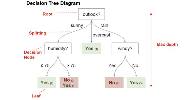
目前了解的最好的决策树图
此时叶子节点中包含的样本类别(或标签均值)为最终的预测结果。这里想要具体的index,也就是样本预测到第几个叶子节点中。
在XGBoost中,拥有多棵树。则一个样本将会被编码为多个index,最终可以将index作为额外的类别特征再加入到模型训练。
具体API
XGBoost
使用Learning API,设置pred_leaf参数
import xgboost as xgb
from sklearn.datasets import make_classification

X, Y = make_classification(1000, 20)
dtrain = xgb.DMatrix(X, Y)
dtest = xgb.DMatrix(X)

param = {'max_depth':10, 'min_child_weight':1, 'learning_rate':0.1}
num_round = 200
bst = xgb.train(param, dtrain, num_round)
bst.predict(dtest, pred_leaf=True)
LightGBM
使用sklearn API或者Learning API,设置pred_leaf参数
-
import lightgbm as lgb -
from sklearn.datasets import make_classification -
X, Y = make_classification(1000, 20) -
dtrain = lgb.Dataset(X, Y) -
dtest = lgb.Dataset(X) -
param = {'max_depth':10, 'min_child_weight':1, 'learning_rate':0.1} -
num_round = 200 -
bst = lgb.train(param, dtrain, num_round) -
bst.predict(X, pred_leaf=True)
CatBoost
使用calc_leaf_indexes函数
-
import catboost as cab -
from sklearn.datasets import make_classification -
X, Y = make_classification(1000, 20) -
clf = cab.CatBoostClassifier(iterations=200) -
clf.fit(X, Y) -
clf.calc_leaf_indexes(X)
使用细节
-
leaf index预测维度与具体树个数相关,也就是与具体的round相关。 -
leaf index的预测结果为类别类型。 -
leaf index建议交叉验证编码,避免自己训练并编码自己。
交叉验证实现:https://www.kaggle.com/mmueller/categorical-embedding-with-xgb/script