弹性变形与采样,旋转,形变场可视化
文章目录
-
- 采样
- (更新)旋转
- 变形场可视化
- 变形与可视化实例
- STN(Spatial Transformer Network)
Dense Deformation(Elastic deformation)的采样与可视化
对于采样(sample)而言,分为前向与后向。前向直观上更容易理解,但实际应用会有问题,因此,算法中的采样操作一般为后向。
采样
前向采样:
- 将输入图像坐标
p1根据DDF(Dense deformation Feild)或Affine Matrix或其他方式进行变换得到坐标p2,输入图像p1坐标处的值 映射到输出图像p2处。
伪代码示例:
#与input_image shape一致的空矩阵
output_image = empty_array()
for row in input_image.height:
	for col in input_image.width:
		# 或者 dx,dy = Affinematrix*[row,col]
		dx,dy = random(),random()
		output_image[row+dy,col+dx] = input_image[row,col]
这样会出现的问题是,output_image中,很多坐标上没有值。而后向采样就能解决这个问题。
后向采样:
- 将输出图像坐标
p1根据DDF(Dense deformation Feild)或Affine Matrix的逆或其他方式进行变换得到坐标p2,输出图像p1坐标处的值 根据输入图像p2坐标处经过插值算法得到的像素值确定。
伪代码示例:
#与input_image shape一致的空矩阵
output_image = empty_array()
for row in output_image.height:
	for col in output_image.width:
		# 或者 dx,dy = Affinematrix_inverse*[row,col]
		dx,dy = random(),random()
		# 根据插值算法,得到input_image中(row+dy,col+dx)处的像素值
		value = interpolate(input_image,row+dy,col+dx)
		output_image[row,col] = value
由伪代码也易看出,后向采样可以确保输出图像中每个坐标都有对应的像素值(若row+dy或col+dx超出输入图像范围,value=None,则是变形的结果,而不是输出图像这一坐标没有值)
(更新)旋转
(2020-6-24)在实现图像旋转时同样遇到了前向采样、后向采样这个问题,觉得很容易弄糊涂,特此记录下自己的一点理解。
已知旋转矩阵(具体推导见后文)为
[ c o s θ − s i n θ s i n θ c o s θ ] \begin{bmatrix} cos\theta &-sin\theta \\ sin\theta& cos\theta \end{bmatrix} [cosθsinθ−sinθcosθ]
其中的 θ \theta θ定义了逆时针旋转的角度(没有特别说明时,旋转中心即图像原点,此处也就是图像左上角)。下面的代码将一个横条旋转了30度。
def warpRotate(image, matrix):
    height, width = image.shape[:2]
    dst = np.zeros((height, width))

    for x in range(height):
        for y in range(width):

            u = int(x*matrix[0,0]+y*matrix[0,1])
            v = int(x*matrix[1,0]+y*matrix[1,1])
           	# 为了直观,这儿用的是前向采样
            if (u >= 0 and u < height) and (v >= 0 and v < width):
                dst[u,v] = image[x,y]
    return dst

#定义原始图像
size = 11
img = np.zeros((size, size))
img[int((size-1)/2), :] = np.ones(size)
#定义旋转矩阵
theta = np.radians(30)
c, s = np.cos(theta), np.sin(theta)
R = np.array(((c, -s), (s, c)))
rotate_img = warpRotate(img,R)
#显示
plt.figure(figsize=(6.4, 4.8), constrained_layout=False)
plt.subplot(121), plt.imshow(img, "gray"), plt.title("origin")
plt.subplot(122), plt.imshow(rotate_img, "gray"), plt.title("rotate img")

由结果能发现,其实所谓旋转,更应该理解成对坐标系进行的旋转,而非内容本身。如下图所示,黑色线为初始坐标,绿色线为旋转后的坐标。其实内容位置相对于局部坐标而言并未改变,只是我们默认原始坐标为全局坐标,也是我们的视野范围,因此旋转矩阵得到实际上是坐标旋转后的内容相对于全局坐标的位置。
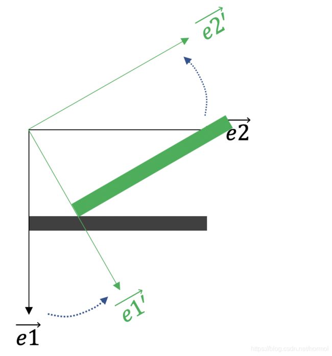
上面的演示代码使用了前向采样,在opencv中,实际上会对矩阵求逆后执行逆向采样,避免如示意图中一样很多空缺像素点(呈现出不平滑状)
旋转矩阵公式推导
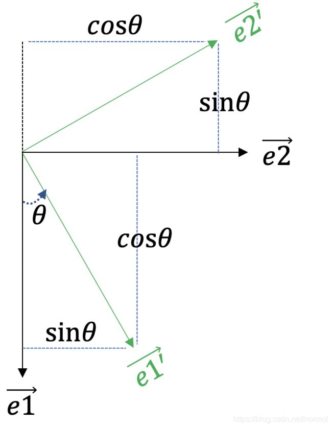
已经知道,所谓旋转即对坐标轴的旋转,而坐标轴实际上是一组基而已,那么由下方的示意图可知,推导公式为:
e 1 ′ ⃗ = c o s θ e 1 ⃗ + s i n θ e 2 ⃗ e 2 ′ ⃗ = − s i n θ e 1 ⃗ + c o s θ e 2 ⃗ \vec{e1'}=cos\theta\vec{e1}+sin\theta\vec{e2}\\ \vec{e2'}=-sin\theta\vec{e1}+cos\theta\vec{e2} e1′=cosθe1+sinθe2e2′=−sinθe1+cosθe2
因此
p ′ = e 1 ′ ⃗ x + e 2 ′ ⃗ y = ( c o s θ − s i n θ ) e 1 ⃗ + ( s i n θ + c o s θ ) e 2 ⃗ p'=\vec{e1'}x+\vec{e2'}y=(cos\theta-sin\theta)\vec{e1}+(sin\theta+cos\theta)\vec{e2} p′=e1′x+e2′y=(cosθ−sinθ)e1+(sinθ+cosθ)e2
p ′ = R p = [ c o s θ − s i n θ s i n θ c o s θ ] ( x y ) p'=Rp=\begin{bmatrix} cos\theta &-sin\theta \\ sin\theta& cos\theta \end{bmatrix}\binom{x}{y} p′=Rp=[cosθsinθ−sinθcosθ](yx)
变形场可视化
这一部分是我自己的思考,不一定正确,若有错误,请指正。
这儿的变形场是针对DDF的,可视化我认为有两种形式,
- 一种是以网格线变形的形式(图1)。第一种形式的可视化我是通过在图像上画线,然后对画了线的图像做变形,最后可视化出来。1 结果自然就能够呈现出网格线变形的效果(不太清楚为什么出现了很多虚线,记得几个月前看过一篇博客说这种原因,以及怎么处理,现在忘记了)。
- 另一种是用箭头可视化变形矢量场(图2)。直接通过
matplotlib的quiver接口实现。(但我认为这儿画的有问题,因为我是通过反向采样实现的变形,例如输入图像(1,1)处的值要变形到输出图像的(2,2)处,根据直观感受来说,此处的箭头应该是位于(1,1)处,指向(2,2)处,但这儿有的数据则是输出图像(2,2)处为(-1,-1),即dx=-1,dy=-1,会表现为出现在(2,2)处指向(1,1)的箭头,虽然可以通过取反调转箭头方向,然而箭尾仍旧出现在(2,2)处)

|

|
变形与可视化实例
环境 python3, jupyter notebook
from scipy.ndimage.interpolation import map_coordinates
from scipy.ndimage.filters import gaussian_filter
import cv2
import numpy as np
import matplotlib.pyplot as plt
%matplotlib inline

def draw_grid(im, grid_size):
    # Draw grid lines
    for i in range(0, im.shape[1], grid_size):
        cv2.line(im, (i, 0), (i, im.shape[0]), color=(1,))
    for j in range(0, im.shape[0], grid_size):
        cv2.line(im, (0, j), (im.shape[1], j), color=(1,))

"""
形式一
"""
image = cv2.imread('./r.jpeg',0)
draw_grid(image,40)

shape = image.shape
sigma = 10
alpha = 180
random_state = np.random.RandomState(1)

dx = gaussian_filter((random_state.rand(*shape) * 2 - 1), sigma) * alpha
dy = gaussian_filter((random_state.rand(*shape) * 2 - 1), sigma) * alpha

x,y = np.meshgrid(np.arange(shape[1]), np.arange(shape[0]))

indices = np.reshape(y+dy, (-1, 1)), np.reshape(x+dx, (-1, 1))
# map_coordinates函数的作用:根据indices中指定的坐标,在image中进行采样
#也就相当于反向采样
image_deform = map_coordinates(image, indices, order=1, mode='reflect').reshape(shape)

plt.imshow(image_deform,cmap='gray')

"""
---------------------------------------------------------------
形式二
"""
image = cv2.imread('./r.jpeg',0)

shape = image.shape
sigma = 10
alpha = 180
random_state = np.random.RandomState(1)

dx = gaussian_filter((random_state.rand(*shape) * 2 - 1), sigma) * alpha
dy = gaussian_filter((random_state.rand(*shape) * 2 - 1), sigma) * alpha

x,y = np.meshgrid(np.arange(shape[1]), np.arange(shape[0]))

# 注意,这儿用np的slice技巧对密集的点进行了下采样,否则画出来的箭头
#完全不能看
plt.quiver(x[::30,::30], y[::30,::30], -dx[::30,::30], -dy[::30,::30],color='red')

indices = np.reshape(y+dy, (-1, 1)), np.reshape(x+dx, (-1, 1))
image_deform = map_coordinates(image, indices, order=2, mode='reflect').reshape(shape)

plt.imshow(image_deform,cmap='gray')
STN(Spatial Transformer Network)
stn作为一个将transform层化的网络,有很多值得学习的地方。这儿提及这个网络,是因为其采样机理就是上面提及过的后向采样(虽然我只看过pytorch的,其余日后有时间看了再补充),涉及两个关键函数F.affine_grid, F.grid_sample2。
用pytorch做小实验的关键部分如下:3
from torch.nn import functional as F
# 这个theta的含义是图像向右平移20%,向下平移40%
theta = torch.tensor([
    [1,0,-0.2],
    [0,1,-0.4]
], dtype=torch.float)
# 修改size
N, C, W, H = img_torch.unsqueeze(0).size()
size = torch.Size((N, C, W//2, H//3))
"""
注意这个grid,经过试验,发现相当于上文出现过的indices,即从输出映射到输入,是反向采样原理。
因为其x方向的输出如下
#print(grid.size()) torch.Size([1, 10, 10, 2])
print(grid[0,:,:,0]) #输出x方向的coordinate
tensor([[-1.2000, -0.9778, -0.7556, -0.5333, -0.3111, -0.0889,  0.1333,  0.3556,
          0.5778,  0.8000],
        [-1.2000, -0.9778, -0.7556, -0.5333, -0.3111, -0.0889,  0.1333,  0.3556,
          0.5778,  0.8000],.......
"""
grid = F.affine_grid(theta.unsqueeze(0), size)
output = F.grid_sample(img_torch.unsqueeze(0), grid)
data-augmentation-with-elastic-deformations ↩︎
Pytorch STN官网示例 ↩︎
Pytorch中的仿射变换(affine_grid) ↩︎