SVM（支持向量机）

目录

前言

一、SVM和KNN

二、SVM分类的代码实现

1.引入库

2.导入数据集

3.构建SVM分类器，训练函数

4.初始化分类器实例，训练模型

5.展示训练结果及验证结果

总结

---

前言

SVM 最早是由 Vladimir N. Vapnik 和 Alexey Ya. Chervonenkis 在1963年提出，目前的版本（soft margin）是由 Corinna Cortes 和 Vapnik 在1993年提出，并在1995年发表。深度学习（2012）出现之前，SVM 被认为机器学习中近十几年来最成功，表现最好的算法。

---

一、SVM和KNN

支持向量机（support vector machines, SVM）是一种二分类模型，它的基本模型是定义在特征空间上的间隔最大的线性分类器，间隔最大使它有别于感知机；SVM还包括核技巧，这使它成为实质上的非线性分类器。SVM的的学习策略就是间隔最大化，可形式化为一个求解凸二次规划的问题，也等价于正则化的合页损失函数的最小化问题。SVM的的学习算法就是求解凸二次规划的最优化算法。

什么是 SVM（支持向量机）？【知多少】_哔哩哔哩_bilibili

KNN(比较一个范围内苹果、梨的多少，来判断样本的种类):

       

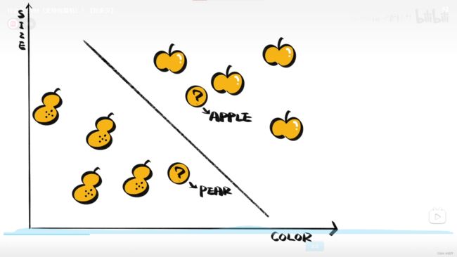
 SVM（通过划定区域来判断所在区域的样本种类）:

 

二、SVM分类的代码实现

1.引入库

import numpy as np
from matplotlib import colors
from sklearn import svm 
from sklearn import model_selection
import matplotlib.pyplot as plt
import matplotlib as mpl

2.导入数据集

def iris_type(s):
    it = {b'Iris-setosa':0, b'Iris-versicolor':1,b'Iris-virginica':2} 
    return it[s]
    
# 1 数据准备
# 1.1 加载数据
data = np.loadtxt('/home/aistudio/data/data2301/iris.data',  # 数据文件路径i
                  dtype=float,    # 数据类型
                  delimiter=',',  # 数据分割符
                  converters={4:iris_type}) # 将第五列使用函数iris_type进行转换
# 1.2 数据分割
x, y = np.split(data, (4, ), axis=1) # 数据分组 第五列开始往后为y 代表纵向分割按列分割
x = x[:, :2]
x_train, x_test, y_train, y_test=model_selection.train_test_split(x, y, random_state=1, test_size=0.2)

3.构建SVM分类器，训练函数

# SVM分类器构建
def classifier():
    clf = svm.SVC(C=0.5,#误差项惩罚系数
                   kernel='rbf',#线性核 kenerl='rbf':高斯核
                   decision_function_shape='ovr')#决策函数
    return clf
    
# 训练模型
def train(clf, x_train, y_train):#导入训练数据，导入分类器参数，进行模型训练
    clf.fit(x_train,#训练集特征向量
            y_train.ravel())#训练集目标值

4.初始化分类器实例，训练模型

# 2 定义模型 SVM模型定义
clf = classifier()
# 3 训练模型
train(clf, x_train, y_train)

5.展示训练结果及验证结果

# ======判断a,b是否相等计算acc的均值
def show_accuracy(a, b, tip):
    acc = a.ravel() == b.ravel()
    print('%s Accuracy:%.3f' %(tip, np.mean(acc)))
    
# 分别打印训练集和测试集的准确率 score(x_train, y_train)表示输出 x_train,y_train在模型上的准确率
def print_accuracy(clf, x_train, y_train, x_test, y_test):
    print('training prediction:%.3f' %(clf.score(x_train, y_train)))
    print('test data prediction:%.3f' %(clf.score(x_test, y_test)))
    # 原始结果和预测结果进行对比 predict() 表示对x_train样本进行预测,返回样本类别
    show_accuracy(clf.predict(x_train), y_train, 'traing data')
    show_accuracy(clf.predict(x_test), y_test, 'testing data')
    # 计算决策函数的值 表示x到各个分割平面的距离
    print('decision_function:\n', clf.decision_function(x_train))
    
def draw(clf, x):   
    iris_feature = 'sepal length', 'sepal width', 'petal length', 'petal width'
    # 开始画图
    x1_min, x1_max = x[:, 0].min(), x[:, 0].max()
    x2_min, x2_max = x[:, 1].min(), x[:, 1].max()
    # 生成网格采样点
    x1, x2 = np.mgrid[x1_min:x1_max:200j, x2_min:x2_max:200j]  
    # 测试点
    grid_test = np.stack((x1.flat, x2.flat), axis = 1)
    print('grid_test:\n', grid_test)
    # 输出样本到决策面的距离
    z = clf.decision_function(grid_test)
    print('the distance to decision plane:\n', z)
    grid_hat = clf.predict(grid_test)
    # 预测分类值 得到[0, 0, ..., 2, 2]
    print('grid_hat:\n', grid_hat)
    # 使得grid_hat 和 x1 形状一致
    grid_hat = grid_hat.reshape(x1.shape)
    cm_light = mpl.colors.ListedColormap(['#A0FFA0', '#FFA0A0', '#A0A0FF'])
    cm_dark = mpl.colors.ListedColormap(['g', 'b', 'r'])
    
    plt.pcolormesh(x1, x2, grid_hat, cmap = cm_light) 
    plt.scatter(x[:, 0], x[:, 1], c=np.squeeze(y), edgecolor='k', s=50, cmap=cm_dark )
    plt.scatter(x_test[:, 0], x_test[:, 1], s=120, facecolor='none', zorder=10 )
    plt.xlabel(iris_feature[0], fontsize=20) # 注意单词的拼写label
    plt.ylabel(iris_feature[1], fontsize=20)
    plt.xlim(x1_min, x1_max)
    plt.ylim(x2_min, x2_max)
    plt.title('Iris data classification via SVM', fontsize=30)
    plt.grid()
    plt.show()

# 4 模型评估
print('-------- eval ----------')
print_accuracy(clf, x_train, y_train, x_test, y_test)
# 5 模型使用
print('-------- show ----------')
draw(clf, x) 

---

总结

SVM代码已经在sklearn中集成，只需确定相应参数即可调用。