线性回归(多重特征)
文章目录
- 1 多重特征Multiple Features
-
- 1.1 向量化Vectorization
- 1.2 代码与效率对比
-
- 1.2.1 向量的创建Vector Creation
- 1.2.2 向量的操作Operations on Vectors
-
- 1.2.2.1 如何索引Indexing
- 1.2.2.2 切片Slicing
- 1.2.2.3 对整个向量操作
- 1.2.2.4 向量之间操作
- 1.2.2.5 标量与向量的操作
- 1.2.2.6 向量点积***
- 1.2.2.7 向量的shape
- 1.2.3 矩阵Matrix的代码表示
-
- 1.2.3.1 创建矩阵Matrix creation
- 1.2.3.2 矩阵索引
- 1.2.3.2 矩阵切片
- 1.3 代码:多特征线性回归Multiple Variable Linear Regression
-
- 1.3.1 房价模型
- 1.3.2 线性回归模型
- 1.3.3 计算cost
- 1.3.4 计算梯度Compute gradient
- 1.3.5 梯度下降Gradient Descent
- 2 梯度下降Gradient descent in practice
-
- 2.1 特征缩放与学习率 Feature scaling and Learning Rate
-
- 2.1.1 学习率 Learning Rate
- 2.1.2 特征缩放Feature scaling
- 2.2 特征工程与多项式回归 Feature Engineering and Polynomial Regression
-
- 2.2.1 多项式回归 Polynomial Regression
- 2.2.2 特征工程Feature Engineering
- 2.2.3 特征缩放 Scaling features
- 2.3 Linear Regression using Scikit-Learn
- 2.4 在线练习(常练常新)

1 多重特征Multiple Features
房价不只size一个特征,还可能有卧室数,地板数,房子年龄.例如
x^(i) = [size, bedrooms, floors, age of home]
可以再加一个下标j表示第几个元素.现在
Subscript[x, j]^(i)表示第i个样例的第j个特征的值.
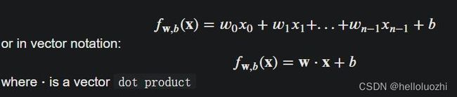
现在多个特征的线性回归模型可写为
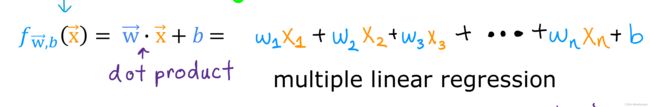
这里w也是向量,b是标量bias.
1.1 向量化Vectorization
我们需要在代码中简洁表示向量点乘,借助NumPy
我们可以把特征feature向量和权重weight向量写为

现在要怎么表达w点积x呢?
用

和

不好,因为代码运行更慢.
直接用np.dao(w,x)

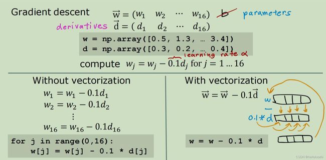
1.2 代码与效率对比
Vectorization后在电脑中计算时并行计算点乘和梯度下降,时间复杂度O(1),比没有Vectorization的O(n)更快.
- 导入
numpy和time(看花费的时间)
import numpy as np
import time
1.2.1 向量的创建Vector Creation
# NumPy routines which allocate memory and fill arrays with value
a = np.zeros(4);                print(f"np.zeros(4) :   a = {a}, a shape = {a.shape}, a data type = {a.dtype}")
a = np.zeros((4,));             print(f"np.zeros(4,) :  a = {a}, a shape = {a.shape}, a data type = {a.dtype}")
a = np.random.random_sample(4); print(f"np.random.random_sample(4): a = {a}, a shape = {a.shape}, a data type = {a.dtype}")


np.zeros(4) :   a = [0. 0. 0. 0.], a shape = (4,), a data type = float64
np.zeros(4,) :  a = [0. 0. 0. 0.], a shape = (4,), a data type = float64
np.random.random_sample(4): a = [0.43105022 0.79710395 0.16488279 0.73185609], a shape = (4,), a data type = float64
zeros元素是零,random是随机
# NumPy routines which allocate memory and fill arrays with value but do not accept shape as input argument
a = np.arange(4.);              print(f"np.arange(4.):     a = {a}, a shape = {a.shape}, a data type = {a.dtype}")
a = np.random.rand(4);          print(f"np.random.rand(4): a = {a}, a shape = {a.shape}, a data type = {a.dtype}")

np.arange(4.):     a = [0. 1. 2. 3.], a shape = (4,), a data type = float64
np.random.rand(4): a = [0.95584264 0.41866986 0.19089539 0.32726125], a shape = (4,), a data type = float64
arange是递增.
# NumPy routines which allocate memory and fill with user specified values
a = np.array([5,4,3,2]);  print(f"np.array([5,4,3,2]):  a = {a},     a shape = {a.shape}, a data type = {a.dtype}")
a = np.array([5.,4,3,2]); print(f"np.array([5.,4,3,2]): a = {a}, a shape = {a.shape}, a data type = {a.dtype}")

np.array([5,4,3,2]):  a = [5 4 3 2],     a shape = (4,), a data type = int64
np.array([5.,4,3,2]): a = [5. 4. 3. 2.], a shape = (4,), a data type = float64
或直接指定.
1.2.2 向量的操作Operations on Vectors
1.2.2.1 如何索引Indexing
和C语言一样,索引是从零开始
#vector indexing operations on 1-D vectors
a = np.arange(10)
print(a)

#access an element
print(f"a[2].shape: {a[2].shape} a[2]  = {a[2]}, Accessing an element returns a scalar")

# access the last element, negative indexes count from the end
print(f"a[-1] = {a[-1]}")

#indexs must be within the range of the vector or they will produce and error
try:
    c = a[10]
except Exception as e:
    print("The error message you'll see is:")
    print(e)

[0 1 2 3 4 5 6 7 8 9]
a[2].shape: () a[2]  = 2, Accessing an element returns a scalar
a[-1] = 9
The error message you'll see is:
index 10 is out of bounds for axis 0 with size 10
1.2.2.2 切片Slicing
切片使用一组三个值 (start:stop:step) 创建一个索引数组。
各种切片:
#vector slicing operations
a = np.arange(10)
print(f"a         = {a}")

#access 5 consecutive elements (start:stop:step)
c = a[2:7:1];     print("a[2:7:1] = ", c)

# access 3 elements separated by two
c = a[2:7:2];     print("a[2:7:2] = ", c)

# access all elements index 3 and above
c = a[3:];        print("a[3:]    = ", c)

# access all elements below index 3
c = a[:3];        print("a[:3]    = ", c)

# access all elements
c = a[:];         print("a[:]     = ", c)

a         = [0 1 2 3 4 5 6 7 8 9]
a[2:7:1] =  [2 3 4 5 6]
a[2:7:2] =  [2 4 6]
a[3:]    =  [3 4 5 6 7 8 9]
a[:3]    =  [0 1 2]
a[:]     =  [0 1 2 3 4 5 6 7 8 9]
1.2.2.3 对整个向量操作
a = np.array([1,2,3,4])
print(f"a             : {a}")
# negate elements of a
b = -a
print(f"b = -a        : {b}")

# sum all elements of a, returns a scalar
b = np.sum(a)
print(f"b = np.sum(a) : {b}")

b = np.mean(a)
print(f"b = np.mean(a): {b}")

b = a**2
print(f"b = a**2      : {b}")

a             : [1 2 3 4]
b = -a        : [-1 -2 -3 -4]
b = np.sum(a) : 10
b = np.mean(a): 2.5
b = a**2      : [ 1  4  9 16]
1.2.2.4 向量之间操作
向量加法
a = np.array([ 1, 2, 3, 4])
b = np.array([-1,-2, 3, 4])
print(f"Binary operators work element wise: {a + b}")

Binary operators work element wise: [0 0 6 8]
加法需要向量一样长
#try a mismatched vector operation
c = np.array([1, 2])
try:
    d = a + c
except Exception as e:
    print("The error message you'll see is:")
    print(e)

The error message you'll see is:
operands could not be broadcast together with shapes (4,) (2,)
1.2.2.5 标量与向量的操作
乘法
a = np.array([1, 2, 3, 4])

# multiply a by a scalar
b = 5 * a
print(f"b = 5 * a : {b}")

b = 5 * a : [ 5 10 15 20]
1.2.2.6 向量点积***
虽然可以写函数用循环实现
定义
def my_dot(a, b):
    """
   Compute the dot product of two vectors

    Args:
      a (ndarray (n,)):  input vector
      b (ndarray (n,)):  input vector with same dimension as a

    Returns:
      x (scalar):
    """
    x=0
    for i in range(a.shape[0]):
        x = x + a[i] * b[i]
    return x
实现
# test 1-D
a = np.array([1, 2, 3, 4])
b = np.array([-1, 4, 3, 2])
print(f"my_dot(a, b) = {my_dot(a, b)}")

my_dot(a, b) = 24
但这个太慢,我们用
# test 1-D
a = np.array([1, 2, 3, 4])
b = np.array([-1, 4, 3, 2])
c = np.dot(a, b)
print(f"NumPy 1-D np.dot(a, b) = {c}, np.dot(a, b).shape = {c.shape} ")
c = np.dot(b, a)
print(f"NumPy 1-D np.dot(b, a) = {c}, np.dot(a, b).shape = {c.shape} ")

NumPy 1-D np.dot(a, b) = 24, np.dot(a, b).shape = ()
NumPy 1-D np.dot(b, a) = 24, np.dot(a, b).shape = ()
np.dot(a, b).shape = () 的括号为空表示是标量
循环更慢的代码证明,对长度一千万的向量:
np.random.seed(1)
a = np.random.rand(10000000)  # very large arrays
b = np.random.rand(10000000)

tic = time.time()  # capture start time
c = np.dot(a, b)
toc = time.time()  # capture end time

print(f"np.dot(a, b) =  {c:.4f}")
print(f"Vectorized version duration: {1000*(toc-tic):.4f} ms ")

tic = time.time()  # capture start time
c = my_dot(a,b)
toc = time.time()  # capture end time

print(f"my_dot(a, b) =  {c:.4f}")
print(f"loop version duration: {1000*(toc-tic):.4f} ms ")

del(a);del(b)  #remove these big arrays from memory

np.dot(a, b) =  2501072.5817
Vectorized version duration: 195.9784 ms
my_dot(a, b) =  2501072.5817
loop version duration: 9432.0059 ms
np.dot用时0.2秒,循环用时9秒!,不同电脑不一样,用时和硬件有关,
np.dot复杂度O(1),循环复杂度O(n)
梯度同理
- NumPy 更好地利用了底层硬件中可用的
数据并行性。 GPU 和现代 CPU 实现了单指令多数据 (SIMD) 管道,允许并行发出多个操作。 这在数据集通常非常大的机器学习中至关重要。
1.2.2.7 向量的shape
shape()中有几个数就是几维张量,0个是标量,1个是向量,2个是矩阵,n个是n维张量.数的值则代表长度.
# show common Course 1 example
X = np.array([[1],[2],[3],[4]])
w = np.array([2])
c = np.dot(X[1], w)

print(f"X[1] has shape {X[1].shape}")
print(f"w has shape {w.shape}")
print(f"c has shape {c.shape}")

X[1] has shape (1,)
w has shape (1,)
c has shape ()
1.2.3 矩阵Matrix的代码表示
X_mn,m是行row,n是列column
1.2.3.1 创建矩阵Matrix creation
2维矩阵,注意np.zeros((3, 1))的形状
a = np.zeros((1, 5))
print(f"a shape = {a.shape}, a = {a}")

a = np.zeros((3, 1))
print(f"a shape = {a.shape}, a = {a}")

a = np.random.random_sample((1, 1))
print(f"a shape = {a.shape}, a = {a}")

a shape = (1, 5), a = [[0. 0. 0. 0. 0.]]
a shape = (3, 1), a = [[0.]
 [0.]
 [0.]]
a shape = (1, 1), a = [[0.77390955]]
指定值:
# NumPy routines which allocate memory and fill with user specified values
a = np.array([[5], [4], [3]]);   print(f" a shape = {a.shape}, np.array: a = {a}")
a = np.array([[5],   # One can also
              [4],   # separate values
              [3]]); #into separate rows
print(f" a shape = {a.shape}, np.array: a = {a}")

 a shape = (3, 1), np.array: a = [[5]
 [4]
 [3]]
 a shape = (3, 1), np.array: a = [[5]
 [4]
 [3]]
1.2.3.2 矩阵索引
.reshape(-1, 2)指的是一行只有两个元素
#vector indexing operations on matrices
a = np.arange(6).reshape(-1, 2)   #reshape is a convenient way to create matrices
print(f"a.shape: {a.shape}, \na= {a}")

#access an element
print(f"\na[2,0].shape:   {a[2, 0].shape}, a[2,0] = {a[2, 0]},     type(a[2,0]) = {type(a[2, 0])} Accessing an element returns a scalar\n")

#access a row
print(f"a[2].shape:   {a[2].shape}, a[2]   = {a[2]}, type(a[2])   = {type(a[2])}")

a.shape: (3, 2),
a= [[0 1]
 [2 3]
 [4 5]]

a[2,0].shape:   (), a[2,0] = 4,     type(a[2,0]) = <class 'numpy.int64'> Accessing an element returns a scalar

a[2].shape:   (2,), a[2]   = [4 5], type(a[2])   = <class 'numpy.ndarray'>
注意索引从0开始,a[2] == [4 5], a[2,0] == 4.仅通过指定行来访问矩阵将返回一维向量
1.2.3.2 矩阵切片
切片使用一组三个值 (start:stop:step) 创建一个索引数组。
#vector 2-D slicing operations
a = np.arange(20).reshape(-1, 10)
print(f"a = \n{a}")

#access 5 consecutive elements (start:stop:step)
print("a[0, 2:7:1] = ", a[0, 2:7:1], ",  a[0, 2:7:1].shape =", a[0, 2:7:1].shape, "a 1-D array")

#access 5 consecutive elements (start:stop:step) in two rows
print("a[:, 2:7:1] = \n", a[:, 2:7:1], ",  a[:, 2:7:1].shape =", a[:, 2:7:1].shape, "a 2-D array")

# access all elements
print("a[:,:] = \n", a[:,:], ",  a[:,:].shape =", a[:,:].shape)

# access all elements in one row (very common usage)
print("a[1,:] = ", a[1,:], ",  a[1,:].shape =", a[1,:].shape, "a 1-D array")
# same as
print("a[1]   = ", a[1],   ",  a[1].shape   =", a[1].shape, "a 1-D array")

a =
[[ 0  1  2  3  4  5  6  7  8  9]
 [10 11 12 13 14 15 16 17 18 19]]
a[0, 2:7:1] =  [2 3 4 5 6] ,  a[0, 2:7:1].shape = (5,) a 1-D array
a[:, 2:7:1] =
 [[ 2  3  4  5  6]
 [12 13 14 15 16]] ,  a[:, 2:7:1].shape = (2, 5) a 2-D array
a[:,:] =
 [[ 0  1  2  3  4  5  6  7  8  9]
 [10 11 12 13 14 15 16 17 18 19]] ,  a[:,:].shape = (2, 10)
a[1,:] =  [10 11 12 13 14 15 16 17 18 19] ,  a[1,:].shape = (10,) a 1-D array
a[1]   =  [10 11 12 13 14 15 16 17 18 19] ,  a[1].shape   = (10,) a 1-D array
1.3 代码:多特征线性回归Multiple Variable Linear Regression
1.3.1 房价模型
代码的表示

我们的模型,预测房价

- 导入
计算和画图
import copy, math
import numpy as np
import matplotlib.pyplot as plt
plt.style.use('./deeplearning.mplstyle')
np.set_printoptions(precision=2)  # reduced display precision on numpy arrays
- 代入数据
X_train = np.array([[2104, 5, 1, 45], [1416, 3, 2, 40], [852, 2, 1, 35]])
y_train = np.array([460, 232, 178])
- 数组都在矩阵中
# data is stored in numpy array/matrix
print(f"X Shape: {X_train.shape}, X Type:{type(X_train)})")
print(X_train)
print(f"y Shape: {y_train.shape}, y Type:{type(y_train)})")
print(y_train)

X Shape: (3, 4), X Type:<class 'numpy.ndarray'>)
[[2104    5    1   45]
 [1416    3    2   40]
 [ 852    2    1   35]]
y Shape: (3,), y Type:<class 'numpy.ndarray'>)
[460 232 178]
1.3.2 线性回归模型
- 起始数据
b_init = 785.1811367994083
w_init = np.array([ 0.39133535, 18.75376741, -53.36032453, -26.42131618])
print(f"w_init shape: {w_init.shape}, b_init type: {type(b_init)}")

w_init shape: (4,), b_init type: <class 'float'>
- 线性回归模型:
- 模型代码
def predict_single_loop(x, w, b):
    """
    single predict using linear regression

    Args:
      x (ndarray): Shape (n,) example with multiple features
      w (ndarray): Shape (n,) model parameters
      b (scalar):  model parameter

    Returns:
      p (scalar):  prediction
    """
    n = x.shape[0]
    p = 0
    for i in range(n):
        p_i = x[i] * w[i]
        p = p + p_i
    p = p + b
    return p
# get a row from our training data
x_vec = X_train[0,:]
print(f"x_vec shape {x_vec.shape}, x_vec value: {x_vec}")

# make a prediction
f_wb = predict_single_loop(x_vec, w_init, b_init)
print(f"f_wb shape {f_wb.shape}, prediction: {f_wb}")

x_vec shape (4,), x_vec value: [2104    5    1   45]
f_wb shape (), prediction: 459.9999976194083
结果是459.9999976194083,实际是460.
- 现在用
.dot
def predict(x, w, b):
    """
    single predict using linear regression
    Args:
      x (ndarray): Shape (n,) example with multiple features
      w (ndarray): Shape (n,) model parameters
      b (scalar):             model parameter

    Returns:
      p (scalar):  prediction
    """
    p = np.dot(x, w) + b
    return p
# get a row from our training data
x_vec = X_train[0,:]
print(f"x_vec shape {x_vec.shape}, x_vec value: {x_vec}")

# make a prediction
f_wb = predict(x_vec,w_init, b_init)
print(f"f_wb shape {f_wb.shape}, prediction: {f_wb}")

x_vec shape (4,), x_vec value: [2104    5    1   45]
f_wb shape (), prediction: 459.99999761940825
结果一样,但predict(x, w, b)比predict_single_loop(x, w, b)更快
1.3.3 计算cost
cost定义
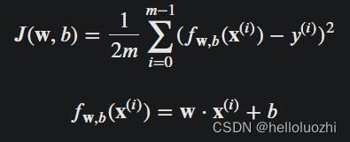
- 代码
def compute_cost(X, y, w, b):
    """
    compute cost
    Args:
      X (ndarray (m,n)): Data, m examples with n features
      y (ndarray (m,)) : target values
      w (ndarray (n,)) : model parameters
      b (scalar)       : model parameter

    Returns:
      cost (scalar): cost
    """
    m = X.shape[0]
    cost = 0.0
    for i in range(m):
        f_wb_i = np.dot(X[i], w) + b           #(n,)(n,) = scalar (see np.dot)
        cost = cost + (f_wb_i - y[i])**2       #scalar
    cost = cost / (2 * m)                      #scalar
    return cost
# Compute and display cost using our pre-chosen optimal parameters.
cost = compute_cost(X_train, y_train, w_init, b_init)
print(f'Cost at optimal w : {cost}')

Cost at optimal w : 1.5578904880036537e-12
最优解.注意w和b已经有了.
1.3.4 计算梯度Compute gradient

- 代码
def compute_gradient(X, y, w, b):
    """
    Computes the gradient for linear regression
    Args:
      X (ndarray (m,n)): Data, m examples with n features
      y (ndarray (m,)) : target values
      w (ndarray (n,)) : model parameters
      b (scalar)       : model parameter

    Returns:
      dj_dw (ndarray (n,)): The gradient of the cost w.r.t. the parameters w.
      dj_db (scalar):       The gradient of the cost w.r.t. the parameter b.
    """
    m,n = X.shape           #(number of examples, number of features)
    dj_dw = np.zeros((n,))
    dj_db = 0.

    for i in range(m):
        err = (np.dot(X[i], w) + b) - y[i]
        for j in range(n):
            dj_dw[j] = dj_dw[j] + err * X[i, j]
        dj_db = dj_db + err
    dj_dw = dj_dw / m
    dj_db = dj_db / m

    return dj_db, dj_dw
注意循环的代码写法, 一个循环每行对齐
- 带入房价模型
#Compute and display gradient
tmp_dj_db, tmp_dj_dw = compute_gradient(X_train, y_train, w_init, b_init)
print(f'dj_db at initial w,b: {tmp_dj_db}')
print(f'dj_dw at initial w,b: \n {tmp_dj_dw}')

dj_db at initial w,b: -1.673925169143331e-06
dj_dw at initial w,b:
 [-2.73e-03 -6.27e-06 -2.22e-06 -6.92e-05]
1.3.5 梯度下降Gradient Descent
def gradient_descent(X, y, w_in, b_in, cost_function, gradient_function, alpha, num_iters):
    """
    Performs batch gradient descent to learn w and b. Updates w and b by taking
    num_iters gradient steps with learning rate alpha

    Args:
      X (ndarray (m,n))   : Data, m examples with n features
      y (ndarray (m,))    : target values
      w_in (ndarray (n,)) : initial model parameters
      b_in (scalar)       : initial model parameter
      cost_function       : function to compute cost
      gradient_function   : function to compute the gradient
      alpha (float)       : Learning rate
      num_iters (int)     : number of iterations to run gradient descent

    Returns:
      w (ndarray (n,)) : Updated values of parameters
      b (scalar)       : Updated value of parameter
      """

    # An array to store cost J and w's at each iteration primarily for graphing later
    J_history = []
    w = copy.deepcopy(w_in)  #avoid modifying global w within function
    b = b_in

    for i in range(num_iters):

        # Calculate the gradient and update the parameters
        dj_db,dj_dw = gradient_function(X, y, w, b)   ##None

        # Update Parameters using w, b, alpha and gradient
        w = w - alpha * dj_dw               ##None
        b = b - alpha * dj_db               ##None

        # Save cost J at each iteration
        if i<100000:      # prevent resource exhaustion
            J_history.append( cost_function(X, y, w, b))

        # Print cost every at intervals 10 times or as many iterations if < 10
        if i% math.ceil(num_iters / 10) == 0:
            print(f"Iteration {i:4d}: Cost {J_history[-1]:8.2f}   ")

    return w, b, J_history #return final w,b and J history for graphing
# initialize parameters
initial_w = np.zeros_like(w_init)
initial_b = 0.
# some gradient descent settings
iterations = 1000
alpha = 5.0e-7
# run gradient descent
w_final, b_final, J_hist = gradient_descent(X_train, y_train, initial_w, initial_b,
                                                    compute_cost, compute_gradient,
                                                    alpha, iterations)
print(f"b,w found by gradient descent: {b_final:0.2f},{w_final} ")
m,_ = X_train.shape
for i in range(m):
    print(f"prediction: {np.dot(X_train[i], w_final) + b_final:0.2f}, target value: {y_train[i]}")

Iteration    0: Cost  2529.46
Iteration  100: Cost   695.99
Iteration  200: Cost   694.92
Iteration  300: Cost   693.86
Iteration  400: Cost   692.81
Iteration  500: Cost   691.77
Iteration  600: Cost   690.73
Iteration  700: Cost   689.71
Iteration  800: Cost   688.70
Iteration  900: Cost   687.69
b,w found by gradient descent: -0.00,[ 0.2   0.   -0.01 -0.07]
prediction: 426.19, target value: 460
prediction: 286.17, target value: 232
prediction: 171.47, target value: 178
# plot cost versus iteration
fig, (ax1, ax2) = plt.subplots(1, 2, constrained_layout=True, figsize=(12, 4))
ax1.plot(J_hist)
ax2.plot(100 + np.arange(len(J_hist[100:])), J_hist[100:])
ax1.set_title("Cost vs. iteration");  ax2.set_title("Cost vs. iteration (tail)")
ax1.set_ylabel('Cost')             ;  ax2.set_ylabel('Cost')
ax1.set_xlabel('iteration step')   ;  ax2.set_xlabel('iteration step')
plt.show()

这些结果并不鼓舞人心! 成本仍在下降,我们的预测不是很准确。 下一个实验室将探索如何改进这一点
2 梯度下降Gradient descent in practice
2.1 特征缩放与学习率 Feature scaling and Learning Rate
2.1.1 学习率 Learning Rate
下面用代码学习多元特征线性回归中如何进行特征缩放和学习率调整
- 配置环境
导入matplotlib和NumPy.
import numpy as np
import matplotlib.pyplot as plt
from lab_utils_multi import  load_house_data, run_gradient_descent
from lab_utils_multi import  norm_plot, plt_equal_scale, plot_cost_i_w
from lab_utils_common import dlc
np.set_printoptions(precision=2)
plt.style.use('./deeplearning.mplstyle')
- 载入房价数据
# load the dataset
X_train, y_train = load_house_data()
X_features = ['size(sqft)','bedrooms','floors','age']
这里load_house_data()的房价数据远超前面,具体如下图:
fig,ax=plt.subplots(1, 4, figsize=(12, 3), sharey=True)
for i in range(len(ax)):
    ax[i].scatter(X_train[:,i],y_train)
    ax[i].set_xlabel(X_features[i])
ax[0].set_ylabel("Price (1000's)")
plt.show()

绘制每个特征与目标价格的关系图,可以表明哪些特征对价格的影响最大。
- 增加尺寸也会增加价格。
- 卧室和地板似乎对价格没有太大影响。
- 新房子的价格高于旧房子。
运用梯度下降,设置学习率为9.9*10^-7:
#set alpha to 9.9e-7
_, _, hist = run_gradient_descent(X_train, y_train, 10, alpha = 9.9e-7)

Iteration Cost          w0       w1       w2       w3       b       djdw0    djdw1    djdw2    djdw3    djdb
---------------------|--------|--------|--------|--------|--------|--------|--------|--------|--------|--------|
        0 9.55884e+04  5.5e-01  1.0e-03  5.1e-04  1.2e-02  3.6e-04 -5.5e+05 -1.0e+03 -5.2e+02 -1.2e+04 -3.6e+02
        1 1.28213e+05 -8.8e-02 -1.7e-04 -1.0e-04 -3.4e-03 -4.8e-05  6.4e+05  1.2e+03  6.2e+02  1.6e+04  4.1e+02
        2 1.72159e+05  6.5e-01  1.2e-03  5.9e-04  1.3e-02  4.3e-04 -7.4e+05 -1.4e+03 -7.0e+02 -1.7e+04 -4.9e+02
        3 2.31358e+05 -2.1e-01 -4.0e-04 -2.3e-04 -7.5e-03 -1.2e-04  8.6e+05  1.6e+03  8.3e+02  2.1e+04  5.6e+02
        4 3.11100e+05  7.9e-01  1.4e-03  7.1e-04  1.5e-02  5.3e-04 -1.0e+06 -1.8e+03 -9.5e+02 -2.3e+04 -6.6e+02
        5 4.18517e+05 -3.7e-01 -7.1e-04 -4.0e-04 -1.3e-02 -2.1e-04  1.2e+06  2.1e+03  1.1e+03  2.8e+04  7.5e+02
        6 5.63212e+05  9.7e-01  1.7e-03  8.7e-04  1.8e-02  6.6e-04 -1.3e+06 -2.5e+03 -1.3e+03 -3.1e+04 -8.8e+02
        7 7.58122e+05 -5.8e-01 -1.1e-03 -6.2e-04 -1.9e-02 -3.4e-04  1.6e+06  2.9e+03  1.5e+03  3.8e+04  1.0e+03
        8 1.02068e+06  1.2e+00  2.2e-03  1.1e-03  2.3e-02  8.3e-04 -1.8e+06 -3.3e+03 -1.7e+03 -4.2e+04 -1.2e+03
        9 1.37435e+06 -8.7e-01 -1.7e-03 -9.1e-04 -2.7e-02 -5.2e-04  2.1e+06  3.9e+03  2.0e+03  5.1e+04  1.4e+03
w,b found by gradient descent: w: [-0.87 -0.   -0.   -0.03], b: -0.00
我们发现w0等的值每次正负不一样,即反复横跳,画出来看:
plot_cost_i_w(X_train, y_train, hist)

右边的图显示了参数之一的值,w0。 在每次迭代中,它都会超过最优值,因此,成本最终会增加而不是接近最小值。 请注意,这不是一张完全准确的图片,因为每次通过都会修改 4 个参数,而不仅仅是一个。 该图仅显示w0,其他参数固定为良性值。 在这个和以后的图中,您可能会注意到蓝色和橙色线略微偏离。
- 现在试一试
更小的学习率
#set alpha to 9e-7
_,_,hist = run_gradient_descent(X_train, y_train, 10, alpha = 9e-7)

Iteration Cost          w0       w1       w2       w3       b       djdw0    djdw1    djdw2    djdw3    djdb
---------------------|--------|--------|--------|--------|--------|--------|--------|--------|--------|--------|
        0 6.64616e+04  5.0e-01  9.1e-04  4.7e-04  1.1e-02  3.3e-04 -5.5e+05 -1.0e+03 -5.2e+02 -1.2e+04 -3.6e+02
        1 6.18990e+04  1.8e-02  2.1e-05  2.0e-06 -7.9e-04  1.9e-05  5.3e+05  9.8e+02  5.2e+02  1.3e+04  3.4e+02
        2 5.76572e+04  4.8e-01  8.6e-04  4.4e-04  9.5e-03  3.2e-04 -5.1e+05 -9.3e+02 -4.8e+02 -1.1e+04 -3.4e+02
        3 5.37137e+04  3.4e-02  3.9e-05  2.8e-06 -1.6e-03  3.8e-05  4.9e+05  9.1e+02  4.8e+02  1.2e+04  3.2e+02
        4 5.00474e+04  4.6e-01  8.2e-04  4.1e-04  8.0e-03  3.2e-04 -4.8e+05 -8.7e+02 -4.5e+02 -1.1e+04 -3.1e+02
        5 4.66388e+04  5.0e-02  5.6e-05  2.5e-06 -2.4e-03  5.6e-05  4.6e+05  8.5e+02  4.5e+02  1.2e+04  2.9e+02
        6 4.34700e+04  4.5e-01  7.8e-04  3.8e-04  6.4e-03  3.2e-04 -4.4e+05 -8.1e+02 -4.2e+02 -9.8e+03 -2.9e+02
        7 4.05239e+04  6.4e-02  7.0e-05  1.2e-06 -3.3e-03  7.3e-05  4.3e+05  7.9e+02  4.2e+02  1.1e+04  2.7e+02
        8 3.77849e+04  4.4e-01  7.5e-04  3.5e-04  4.9e-03  3.2e-04 -4.1e+05 -7.5e+02 -3.9e+02 -9.1e+03 -2.7e+02
        9 3.52385e+04  7.7e-02  8.3e-05 -1.1e-06 -4.2e-03  8.9e-05  4.0e+05  7.4e+02  3.9e+02  1.0e+04  2.5e+02
w,b found by gradient descent: w: [ 7.74e-02  8.27e-05 -1.06e-06 -4.20e-03], b: 0.00
plot_cost_i_w(X_train, y_train, hist)

在左侧,您会看到成本正在下降。 在右侧,您可以看到w0 仍在最小值附近振荡,但它在每次迭代中都在减少而不是增加。 请注意,当 w[0] 跳过最佳值时,dj_dw[0] 会随着每次迭代而改变符号。 这个 alpha 值将收敛。 您可以改变迭代次数以查看其行为方式。
- 现在试一试
更小的学习率
#set alpha to 1e-7
_,_,hist = run_gradient_descent(X_train, y_train, 10, alpha = 1e-7)

Iteration Cost          w0       w1       w2       w3       b       djdw0    djdw1    djdw2    djdw3    djdb
---------------------|--------|--------|--------|--------|--------|--------|--------|--------|--------|--------|
        0 4.42313e+04  5.5e-02  1.0e-04  5.2e-05  1.2e-03  3.6e-05 -5.5e+05 -1.0e+03 -5.2e+02 -1.2e+04 -3.6e+02
        1 2.76461e+04  9.8e-02  1.8e-04  9.2e-05  2.2e-03  6.5e-05 -4.3e+05 -7.9e+02 -4.0e+02 -9.5e+03 -2.8e+02
        2 1.75102e+04  1.3e-01  2.4e-04  1.2e-04  2.9e-03  8.7e-05 -3.4e+05 -6.1e+02 -3.1e+02 -7.3e+03 -2.2e+02
        3 1.13157e+04  1.6e-01  2.9e-04  1.5e-04  3.5e-03  1.0e-04 -2.6e+05 -4.8e+02 -2.4e+02 -5.6e+03 -1.8e+02
        4 7.53002e+03  1.8e-01  3.3e-04  1.7e-04  3.9e-03  1.2e-04 -2.1e+05 -3.7e+02 -1.9e+02 -4.2e+03 -1.4e+02
        5 5.21639e+03  2.0e-01  3.5e-04  1.8e-04  4.2e-03  1.3e-04 -1.6e+05 -2.9e+02 -1.5e+02 -3.1e+03 -1.1e+02
        6 3.80242e+03  2.1e-01  3.8e-04  1.9e-04  4.5e-03  1.4e-04 -1.3e+05 -2.2e+02 -1.1e+02 -2.3e+03 -8.6e+01
        7 2.93826e+03  2.2e-01  3.9e-04  2.0e-04  4.6e-03  1.4e-04 -9.8e+04 -1.7e+02 -8.6e+01 -1.7e+03 -6.8e+01
        8 2.41013e+03  2.3e-01  4.1e-04  2.1e-04  4.7e-03  1.5e-04 -7.7e+04 -1.3e+02 -6.5e+01 -1.2e+03 -5.4e+01
        9 2.08734e+03  2.3e-01  4.2e-04  2.1e-04  4.8e-03  1.5e-04 -6.0e+04 -1.0e+02 -4.9e+01 -7.5e+02 -4.3e+01
w,b found by gradient descent: w: [2.31e-01 4.18e-04 2.12e-04 4.81e-03], b: 0.00
plot_cost_i_w(X_train,y_train,hist)

在左侧,您会看到成本正在下降。 在右侧,您可以看到w0 在不超过最小值的情况下减少。 请注意,在整个运行过程中 dj_w0 为负数。 此解决方案也将收敛,尽管不如前面的示例那么快。
- 总截图:

2.1.2 特征缩放Feature scaling
重新缩放数据集以使特征具有相似范围是重要的:

有三种缩放:
特征缩放,本质上是将每个正特征除以其最大值,或者更一般地,使用(x-min)/(max-min)将每个特征重新缩放为其最小值和最大值。 两种方法都将特征归一化到-1 和 1的范围内,其中前一种方法适用于正向特征,这很简单,非常适合讲座的示例,而后一种方法适用于任何特征- 均值归一化Mean normalization:
:=(−)/(−) - Z-score归一化:

对特征进行归一化时,重要的是存储用于归一化的值 - 用于计算的平均值和标准偏差。 在从模型中学习到参数之后,我们经常想要预测我们以前没见过的房子的价格。 给定一个新的 x 值(客厅面积和卧室数量),我们必须首先使用我们之前从训练集计算的均值和标准差对 x 进行归一化。 - Z-score归一化的代码:
def zscore_normalize_features(X):
    """
    computes  X, zcore normalized by column

    Args:
      X (ndarray (m,n))     : input data, m examples, n features

    Returns:
      X_norm (ndarray (m,n)): input normalized by column
      mu (ndarray (n,))     : mean of each feature
      sigma (ndarray (n,))  : standard deviation of each feature
    """
    # find the mean of each column/feature
    mu     = np.mean(X, axis=0)                 # mu will have shape (n,)
    # find the standard deviation of each column/feature
    sigma  = np.std(X, axis=0)                  # sigma will have shape (n,)
    # element-wise, subtract mu for that column from each example, divide by std for that column
    X_norm = (X - mu) / sigma

    return (X_norm, mu, sigma)

#check our work
#from sklearn.preprocessing import scale
#scale(X_orig, axis=0, with_mean=True, with_std=True, copy=True)
- 具体实现Z-score:
mu     = np.mean(X_train,axis=0)
sigma  = np.std(X_train,axis=0)
X_mean = (X_train - mu)
X_norm = (X_train - mu)/sigma

fig,ax=plt.subplots(1, 3, figsize=(12, 3))
ax[0].scatter(X_train[:,0], X_train[:,3])
ax[0].set_xlabel(X_features[0]); ax[0].set_ylabel(X_features[3]);
ax[0].set_title("unnormalized")
ax[0].axis('equal')

ax[1].scatter(X_mean[:,0], X_mean[:,3])
ax[1].set_xlabel(X_features[0]); ax[0].set_ylabel(X_features[3]);
ax[1].set_title(r"X - $\mu$")
ax[1].axis('equal')

ax[2].scatter(X_norm[:,0], X_norm[:,3])
ax[2].set_xlabel(X_features[0]); ax[0].set_ylabel(X_features[3]);
ax[2].set_title(r"Z-score normalized")
ax[2].axis('equal')
plt.tight_layout(rect=[0, 0.03, 1, 0.95])
fig.suptitle("distribution of features before, during, after normalization")
plt.show()

上图显示了两个训练集参数“age”和“size(sqft)”之间的关系。 这些以相同的比例绘制。
-
左:未归一化:‘size(sqft)’ 特征的值范围或方差远大于年龄
-
中:第一步从
每个特征中移除均值或平均值。 这会留下以零为中心的特征。 很难看出“年龄”特征的差异,但“尺寸(平方英尺)”显然在零附近。 -
右:第二步
除以标准差。 这使得两个特征都以零为中心,具有相似的比例。 -
让我们对数据进行归一化并将其与原始数据进行比较。
# normalize the original features
X_norm, X_mu, X_sigma = zscore_normalize_features(X_train)
print(f"X_mu = {X_mu}, \nX_sigma = {X_sigma}")
print(f"Peak to Peak range by column in Raw        X:{np.ptp(X_train,axis=0)}")
print(f"Peak to Peak range by column in Normalized X:{np.ptp(X_norm,axis=0)}")

X_mu = [1.42e+03 2.72e+00 1.38e+00 3.84e+01],
X_sigma = [411.62   0.65   0.49  25.78]
Peak to Peak range by column in Raw        X:[2.41e+03 4.00e+00 1.00e+00 9.50e+01]
Peak to Peak range by column in Normalized X:[5.85 6.14 2.06 3.69]
注意Peak to Peak range by column in Normalized X:[5.85 6.14 2.06 3.69],下面画图:
fig,ax=plt.subplots(1, 4, figsize=(12, 3))
for i in range(len(ax)):
    norm_plot(ax[i],X_train[:,i],)
    ax[i].set_xlabel(X_features[i])
ax[0].set_ylabel("count");
fig.suptitle("distribution of features before normalization")
plt.show()
fig,ax=plt.subplots(1,4,figsize=(12,3))
for i in range(len(ax)):
    norm_plot(ax[i],X_norm[:,i],)
    ax[i].set_xlabel(X_features[i])
ax[0].set_ylabel("count");
fig.suptitle("distribution of features after normalization")

plt.show()

通过归一化,每根色谱柱的峰间范围从数千倍减少到 2-3 倍。归一化数据的范围(x 轴)以零为中心.
- 现在我们
已经归一化了,可以进行梯度下降:
w_norm, b_norm, hist = run_gradient_descent(X_norm, y_train, 1000, 1.0e-1, )

Iteration Cost          w0       w1       w2       w3       b       djdw0    djdw1    djdw2    djdw3    djdb
---------------------|--------|--------|--------|--------|--------|--------|--------|--------|--------|--------|
        0 5.76170e+04  8.9e+00  3.0e+00  3.3e+00 -6.0e+00  3.6e+01 -8.9e+01 -3.0e+01 -3.3e+01  6.0e+01 -3.6e+02
      100 2.21086e+02  1.1e+02 -2.0e+01 -3.1e+01 -3.8e+01  3.6e+02 -9.2e-01  4.5e-01  5.3e-01 -1.7e-01 -9.6e-03
      200 2.19209e+02  1.1e+02 -2.1e+01 -3.3e+01 -3.8e+01  3.6e+02 -3.0e-02  1.5e-02  1.7e-02 -6.0e-03 -2.6e-07
      300 2.19207e+02  1.1e+02 -2.1e+01 -3.3e+01 -3.8e+01  3.6e+02 -1.0e-03  5.1e-04  5.7e-04 -2.0e-04 -6.9e-12
      400 2.19207e+02  1.1e+02 -2.1e+01 -3.3e+01 -3.8e+01  3.6e+02 -3.4e-05  1.7e-05  1.9e-05 -6.6e-06 -2.7e-13
      500 2.19207e+02  1.1e+02 -2.1e+01 -3.3e+01 -3.8e+01  3.6e+02 -1.1e-06  5.6e-07  6.2e-07 -2.2e-07 -2.6e-13
      600 2.19207e+02  1.1e+02 -2.1e+01 -3.3e+01 -3.8e+01  3.6e+02 -3.7e-08  1.9e-08  2.1e-08 -7.3e-09 -2.6e-13
      700 2.19207e+02  1.1e+02 -2.1e+01 -3.3e+01 -3.8e+01  3.6e+02 -1.2e-09  6.2e-10  6.9e-10 -2.4e-10 -2.6e-13
      800 2.19207e+02  1.1e+02 -2.1e+01 -3.3e+01 -3.8e+01  3.6e+02 -4.1e-11  2.1e-11  2.3e-11 -8.1e-12 -2.7e-13
      900 2.19207e+02  1.1e+02 -2.1e+01 -3.3e+01 -3.8e+01  3.6e+02 -1.4e-12  7.0e-13  7.6e-13 -2.7e-13 -2.6e-13
w,b found by gradient descent: w: [110.56 -21.27 -32.71 -37.97], b: 363.16
缩放后的特征可以更快地获得非常准确的结果! 请注意,在这个相当短的运行结束时,每个参数的梯度都很小。 0.1 的学习率是使用归一化特征回归的良好开端。 让我们绘制我们的预测与目标值。 请注意,预测是使用归一化特征进行的,而绘图是使用原始特征值显示的。
#predict target using normalized features
m = X_norm.shape[0]
yp = np.zeros(m)
for i in range(m):
    yp[i] = np.dot(X_norm[i], w_norm) + b_norm

    # plot predictions and targets versus original features
fig,ax=plt.subplots(1,4,figsize=(12, 3),sharey=True)
for i in range(len(ax)):
    ax[i].scatter(X_train[:,i],y_train, label = 'target')
    ax[i].set_xlabel(X_features[i])
    ax[i].scatter(X_train[:,i],yp,color=dlc["dlorange"], label = 'predict')
ax[0].set_ylabel("Price"); ax[0].legend();
fig.suptitle("target versus prediction using z-score normalized model")
plt.show()

- 有了多个特征,我们不能再用一个图来显示结果与特征。
- 生成图时,使用了归一化特征。 任何使用从归一化训练集中学习到的参数的预测也必须进行归一化。
- 现在进行预测:
预测 生成我们的模型的目的是用它来预测不在数据集中的房价。让我们预测一栋 1200 平方英尺、3 间卧室、1 层、40 年历史的房子的价格。 回想一下,您必须使用对训练数据进行归一化时得出的均值和标准差对数据进行归一化。
# First, normalize out example.
x_house = np.array([1200, 3, 1, 40])
x_house_norm = (x_house - X_mu) / X_sigma
print(x_house_norm)
x_house_predict = np.dot(x_house_norm, w_norm) + b_norm
print(f" predicted price of a house with 1200 sqft, 3 bedrooms, 1 floor, 40 years old = ${x_house_predict*1000:0.0f}")

[-0.53  0.43 -0.79  0.06]
 predicted price of a house with 1200 sqft, 3 bedrooms, 1 floor, 40 years old = $318709
归一化后的轮廓图是圆的,不是下图的上面这种椭圆!

结论:
- 利用您在以前的实验室中开发的具有多个特征的线性回归例程
- 探索学习率 α 对收敛的影响
- 发现使用 z-score 归一化的特征缩放在加速收敛中的价值
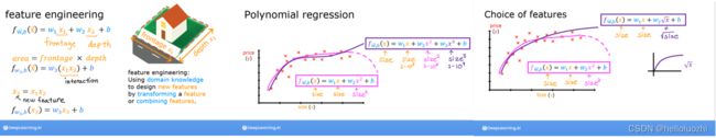
2.2 特征工程与多项式回归 Feature Engineering and Polynomial Regression
探索特征工程和多项式回归,它允许您使用线性回归机制来拟合非常复杂甚至非常非线性的函数
- 工具包
import numpy as np
import matplotlib.pyplot as plt
from lab_utils_multi import zscore_normalize_features, run_gradient_descent_feng
np.set_printoptions(precision=2)  # reduced display precision on numpy arrays
开箱即用,线性回归提供了一种构建模型的方法
![]()
如果您的特征/数据是非线性的或者是特征的组合怎么办? 例如,房价不倾向于与居住面积成线性关系,而是会惩罚非常小或非常大的房屋,从而导致上图所示的曲线。 我们如何使用线性回归机制来拟合这条曲线? 回想一下,我们拥有的“机器”是能够修改(1)中的参数 , 以将方程“拟合”到训练数据。 然而,在 (1) 中对 和 的任何调整都无法实现对非线性曲线的拟合。
2.2.1 多项式回归 Polynomial Regression
上面我们正在考虑数据是非线性的情况。 让我们尝试使用我们目前所知道的来拟合非线性曲线。 我们将从一个简单的二次方程开始:
=1+**2
您熟悉我们使用的所有例程。 它们在 lab_utils.py 文件中可供查看。 我们将使用 np.c_[…] 这是一个 NumPy 例程沿列边界连接。
拟合一个二次曲线
# create target data
x = np.arange(0, 20, 1)
y = 1 + x**2
X = x.reshape(-1, 1)

model_w,model_b = run_gradient_descent_feng(X,y,iterations=1000, alpha = 1e-2)

plt.scatter(x, y, marker='x', c='r', label="Actual Value"); plt.title("no feature engineering")
plt.plot(x,X@model_w + model_b, label="Predicted Value");  plt.xlabel("X"); plt.ylabel("y"); plt.legend()

Iteration         0, Cost: 1.65756e+03
Iteration       100, Cost: 6.94549e+02
Iteration       200, Cost: 5.88475e+02
Iteration       300, Cost: 5.26414e+02
Iteration       400, Cost: 4.90103e+02
Iteration       500, Cost: 4.68858e+02
Iteration       600, Cost: 4.56428e+02
Iteration       700, Cost: 4.49155e+02
Iteration       800, Cost: 4.44900e+02
Iteration       900, Cost: 4.42411e+02
w,b found by gradient descent: w: [18.7], b: -52.0834

正如预期的那样,用直线拟合二次曲线不是很合适。 需要的是类似 =0**2 + b 或多项式特征。 为此,您可以修改输入数据以设计所需的功能。
# create target data
x = np.arange(0, 20, 1)
y = 1 + x**2

# Engineer features
X = x**2      #<-- added engineered feature
注意X = x**2 ,特征已换为二次,不再是线性
X = X.reshape(-1, 1)  #X should be a 2-D Matrix
model_w,model_b = run_gradient_descent_feng(X, y, iterations=10000, alpha = 1e-5)

plt.scatter(x, y, marker='x', c='r', label="Actual Value"); plt.title("Added x**2 feature")
plt.plot(x, np.dot(X,model_w) + model_b, label="Predicted Value"); plt.xlabel("x"); plt.ylabel("y"); plt.legend(); plt.show()

Iteration         0, Cost: 7.32922e+03
Iteration      1000, Cost: 2.24844e-01
Iteration      2000, Cost: 2.22795e-01
Iteration      3000, Cost: 2.20764e-01
Iteration      4000, Cost: 2.18752e-01
Iteration      5000, Cost: 2.16758e-01
Iteration      6000, Cost: 2.14782e-01
Iteration      7000, Cost: 2.12824e-01
Iteration      8000, Cost: 2.10884e-01
Iteration      9000, Cost: 2.08962e-01
w,b found by gradient descent: w: [1.], b: 0.0490
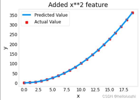
拟合得很好! y=1*x**2+0.049,真实的是y=1*x**2 + 1.很接近.
2.2.2 特征工程Feature Engineering
其实特征的选择不一定提前就知道,上面的模型也有可能采取为:

# create target data
x = np.arange(0, 20, 1)
y = x**2

# engineer features .
X = np.c_[x, x**2, x**3]   #<-- added engineered feature
model_w,model_b = run_gradient_descent_feng(X, y, iterations=10000, alpha=1e-7)

plt.scatter(x, y, marker='x', c='r', label="Actual Value"); plt.title("x, x**2, x**3 features")
plt.plot(x, X@model_w + model_b, label="Predicted Value"); plt.xlabel("x"); plt.ylabel("y"); plt.legend(); plt.show()

Iteration         0, Cost: 1.14029e+03
Iteration      1000, Cost: 3.28539e+02
Iteration      2000, Cost: 2.80443e+02
Iteration      3000, Cost: 2.39389e+02
Iteration      4000, Cost: 2.04344e+02
Iteration      5000, Cost: 1.74430e+02
Iteration      6000, Cost: 1.48896e+02
Iteration      7000, Cost: 1.27100e+02
Iteration      8000, Cost: 1.08495e+02
Iteration      9000, Cost: 9.26132e+01
w,b found by gradient descent: w: [0.08 0.54 0.03], b: 0.0106

拟合的公式是

很明显x**2的系数w1的值最大,其影响最大.梯度下降通过强调其相关参数为我们挑选“正确”的特征.
最初,这些特征被重新缩放,因此它们可以相互比较.较小的权重值意味着不太重要/正确的特征,并且在极端情况下,当权重变为零或非常接近于零时,相关特征在将模型拟合到数据时没有用。上面,在拟合之后,与 **2 特征相关的权重远大于 或 **3 的权重,因为它在拟合数据时最有用。
- 一种观点认为,
特征feature对于目标target应该是线性linear的
# create target data
x = np.arange(0, 20, 1)
y = x**2

# engineer features .
X = np.c_[x, x**2, x**3]   #<-- added engineered feature
X_features = ['x','x^2','x^3']
fig,ax=plt.subplots(1, 3, figsize=(12, 3), sharey=True)
for i in range(len(ax)):
    ax[i].scatter(X[:,i],y)
    ax[i].set_xlabel(X_features[i])
ax[0].set_ylabel("y")
plt.show()

上面,很明显,映射到目标值 y 的 x**2 特征是线性的。 然后,线性回归可以使用该特征轻松生成模型。
2.2.3 特征缩放 Scaling features
如上一个实验所述,如果数据集的特征具有显着不同的尺度,则应该应用特征尺度来加速梯度下降。 在上面的例子中,有x、x2 和x3,它们自然会有非常不同的尺度。 让我们将 Z 分数归一化应用于我们的示例。
# create target data
x = np.arange(0,20,1)
X = np.c_[x, x**2, x**3]
print(f"Peak to Peak range by column in Raw        X:{np.ptp(X,axis=0)}")

# add mean_normalization
X = zscore_normalize_features(X)
print(f"Peak to Peak range by column in Normalized X:{np.ptp(X,axis=0)}")

Peak to Peak range by column in Raw        X:[  19  361 6859]
Peak to Peak range by column in Normalized X:[3.3  3.18 3.28]
x = np.arange(0,20,1)
y = x**2

X = np.c_[x, x**2, x**3]
X = zscore_normalize_features(X)

model_w, model_b = run_gradient_descent_feng(X, y, iterations=100000, alpha=1e-1)

plt.scatter(x, y, marker='x', c='r', label="Actual Value"); plt.title("Normalized x x**2, x**3 feature")
plt.plot(x,X@model_w + model_b, label="Predicted Value"); plt.xlabel("x"); plt.ylabel("y"); plt.legend(); plt.show()

Iteration         0, Cost: 9.42147e+03
Iteration     10000, Cost: 3.90938e-01
Iteration     20000, Cost: 2.78389e-02
Iteration     30000, Cost: 1.98242e-03
Iteration     40000, Cost: 1.41169e-04
Iteration     50000, Cost: 1.00527e-05
Iteration     60000, Cost: 7.15855e-07
Iteration     70000, Cost: 5.09763e-08
Iteration     80000, Cost: 3.63004e-09
Iteration     90000, Cost: 2.58497e-10
w,b found by gradient descent: w: [5.27e-05 1.13e+02 8.43e-05], b: 123.5000
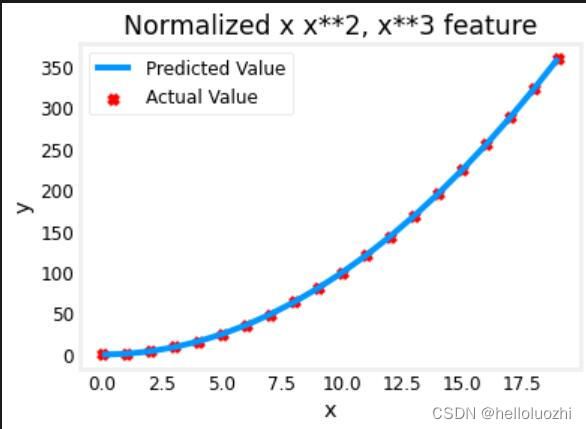
w: [5.27e-05 1.13e+02 8.43e-05]
特征缩放允许它更快地收敛。 再次注意 w 的值。 w1 项,即x2 项是最强调的。 梯度下降几乎消除了x3 项。
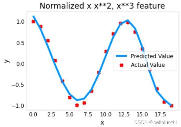
- 我们甚至可以用
多项式特征来拟合三角函数等复制函数
x = np.arange(0,20,1)
y = np.cos(x/2)

X = np.c_[x, x**2, x**3,x**4, x**5, x**6, x**7, x**8, x**9, x**10, x**11, x**12, x**13]
X = zscore_normalize_features(X)

model_w,model_b = run_gradient_descent_feng(X, y, iterations=1000000, alpha = 1e-1)

plt.scatter(x, y, marker='x', c='r', label="Actual Value"); plt.title("Normalized x x**2, x**3 feature")
plt.plot(x,X@model_w + model_b, label="Predicted Value"); plt.xlabel("x"); plt.ylabel("y"); plt.legend(); plt.show()

Iteration         0, Cost: 2.20188e-01
Iteration    100000, Cost: 1.70074e-02
Iteration    200000, Cost: 1.27603e-02
Iteration    300000, Cost: 9.73032e-03
Iteration    400000, Cost: 7.56440e-03
Iteration    500000, Cost: 6.01412e-03
Iteration    600000, Cost: 4.90251e-03
Iteration    700000, Cost: 4.10351e-03
Iteration    800000, Cost: 3.52730e-03
Iteration    900000, Cost: 3.10989e-03
w,b found by gradient descent: w: [ -1.34 -10.    24.78   5.96 -12.49 -16.26  -9.51   0.59   8.7   11.94
   9.27   0.79 -12.82], b: -0.0073
2.3 Linear Regression using Scikit-Learn
有一个开源的、商业上可用的机器学习工具包,称为 scikit-learn。 该工具包包含许多算法的实现。
利用 scikit-learn 使用梯度下降实现线性回归,导入包:
import numpy as np
import matplotlib.pyplot as plt
from sklearn.linear_model import SGDRegressor
from sklearn.preprocessing import StandardScaler
from lab_utils_multi import  load_house_data
from lab_utils_common import dlc
np.set_printoptions(precision=2)
plt.style.use('./deeplearning.mplstyle')
Scikit-learn 有一个梯度下降回归模型 sklearn.linear_model.SGDRegressor。 就像你之前的梯度下降实现一样,这个模型在归一化输入的情况下表现最好。 sklearn.preprocessing.StandardScaler 将像之前的实验室一样执行 z 分数标准化。 在这里,它被称为“标准分数”。
- 导入房价:
X_train, y_train = load_house_data()
X_features = ['size(sqft)','bedrooms','floors','age']
- 归一化数据集
scaler = StandardScaler()
X_norm = scaler.fit_transform(X_train)
print(f"Peak to Peak range by column in Raw        X:{np.ptp(X_train,axis=0)}")
print(f"Peak to Peak range by column in Normalized X:{np.ptp(X_norm,axis=0)}")

Peak to Peak range by column in Raw        X:[2.41e+03 4.00e+00 1.00e+00 9.50e+01]
Peak to Peak range by column in Normalized X:[5.85 6.14 2.06 3.69]
- 创建回归模型并拟合
sgdr = SGDRegressor(max_iter=1000)
sgdr.fit(X_norm, y_train)
print(sgdr)
print(f"number of iterations completed: {sgdr.n_iter_}, number of weight updates: {sgdr.t_}")

SGDRegressor(alpha=0.0001, average=False, early_stopping=False, epsilon=0.1,
             eta0=0.01, fit_intercept=True, l1_ratio=0.15,
             learning_rate='invscaling', loss='squared_loss', max_iter=1000,
             n_iter_no_change=5, penalty='l2', power_t=0.25, random_state=None,
             shuffle=True, tol=0.001, validation_fraction=0.1, verbose=0,
             warm_start=False)
number of iterations completed: 132, number of weight updates: 13069.0
View parameters
- 拟合数据
b_norm = sgdr.intercept_
w_norm = sgdr.coef_
print(f"model parameters:                   w: {w_norm}, b:{b_norm}")
print( "model parameters from previous lab: w: [110.56 -21.27 -32.71 -37.97], b: 363.16")

model parameters:                   w: [110.24 -21.11 -32.51 -38.05], b:[363.17]
model parameters from previous lab: w: [110.56 -21.27 -32.71 -37.97], b: 363.16
请注意,参数与归一化的输入数据相关联。 拟合参数非常接近之前实验室中使用此数据发现的参数。
- 预测
# make a prediction using sgdr.predict()
y_pred_sgd = sgdr.predict(X_norm)
# make a prediction using w,b.
y_pred = np.dot(X_norm, w_norm) + b_norm
print(f"prediction using np.dot() and sgdr.predict match: {(y_pred == y_pred_sgd).all()}")

print(f"Prediction on training set:\n{y_pred[:4]}" )
print(f"Target values \n{y_train[:4]}")

prediction using np.dot() and sgdr.predict match: True
Prediction on training set:
[295.16 485.96 389.6  492.12]
Target values
[300.  509.8 394.  540. ]
- 图
# plot predictions and targets vs original features
fig,ax=plt.subplots(1,4,figsize=(12,3),sharey=True)
for i in range(len(ax)):
    ax[i].scatter(X_train[:,i],y_train, label = 'target')
    ax[i].set_xlabel(X_features[i])
    ax[i].scatter(X_train[:,i],y_pred,color=dlc["dlorange"], label = 'predict')
ax[0].set_ylabel("Price"); ax[0].legend();
fig.suptitle("target versus prediction using z-score normalized model")
plt.show()

2.4 在线练习(常练常新)
在线练习Linear Regression