PCA降维 小白实战初探
记录利用PCA主成分分析法对python自带的鸢尾花数据集进行降维的过程,没有直接的调用PCA库,而是用协方差矩阵一步一步算的,利于加深印象,方便以后复习~
导库导数据
#PCA降维鸢尾花实战
import numpy as np
import pandas as pd
df = pd.read_csv('iris.data')
df.columns=['sepal_len', 'sepal_wid', 'petal_len', 'petal_wid', 'class'] #赋标签

# split data table into data X and class labels y

#此处注意新库不支持df.ix,要改成df.iloc才能正常运行
X = df.iloc[:,0:4].values
y = df.iloc[:,4].values
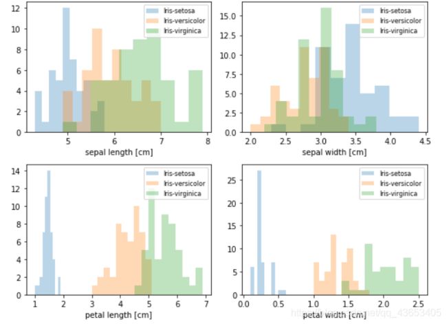
#做之前先直观感受下各指标的变化情况
from matplotlib import pyplot as plt
import math

label_dict = {1: 'Iris-Setosa',
              2: 'Iris-Versicolor',
              3: 'Iris-Virgnica'}

feature_dict = {0: 'sepal length [cm]',
                1: 'sepal width [cm]',
                2: 'petal length [cm]',
                3: 'petal width [cm]'}


plt.figure(figsize=(8, 6))
for cnt in range(4):
    plt.subplot(2, 2, cnt+1)
    for lab in ('Iris-setosa', 'Iris-versicolor', 'Iris-virginica'):
        plt.hist(X[y==lab, cnt],
                     label=lab,
                     bins=10,
                     alpha=0.3,)
    plt.xlabel(feature_dict[cnt])
    plt.legend(loc='upper right', fancybox=True, fontsize=8)

plt.tight_layout()
plt.show()
下面进行PCA处理:
#首先进行0~1标准化处理
from sklearn.preprocessing import StandardScaler
X_std = StandardScaler().fit_transform(X)
mean_vec = np.mean(X_std, axis=0) #均值向量
cov_mat = (X_std - mean_vec).T.dot((X_std - mean_vec)) / (X_std.shape[0]-1)  #得到协方差矩阵
print('Covariance matrix \n%s' %cov_mat)
Covariance matrix
[[ 1.00675676 -0.10448539 0.87716999 0.82249094]
[-0.10448539 1.00675676 -0.41802325 -0.35310295]
[ 0.87716999 -0.41802325 1.00675676 0.96881642]
[ 0.82249094 -0.35310295 0.96881642 1.00675676]]
#计算特征值和特征向量
eig_vals, eig_vecs = np.linalg.eig(cov_mat)
print('Eigenvectors \n%s' %eig_vecs)
print('\nEigenvalues \n%s' %eig_vals)
Eigenvectors
[[ 0.52308496 -0.36956962 -0.72154279 0.26301409]
[-0.25956935 -0.92681168 0.2411952 -0.12437342]
[ 0.58184289 -0.01912775 0.13962963 -0.80099722]
[ 0.56609604 -0.06381646 0.63380158 0.52321917]]
Eigenvalues
[2.92442837 0.93215233 0.14946373 0.02098259]
# Make a list of (eigenvalue, eigenvector) tuples
#1个特征值对应一个特征向量
eig_pairs = [(np.abs(eig_vals[i]), eig_vecs[:,i]) for i in range(len(eig_vals))]
print (eig_pairs)
print ('----------')
# Sort the (eigenvalue, eigenvector) tuples from high to low
eig_pairs.sort(key=lambda x: x[0], reverse=True)

# Visually confirm that the list is correctly sorted by decreasing eigenvalues
#排序特征值
print('Eigenvalues in descending order:')
for i in eig_pairs:
    print(i[0])

#用两个选取的特征向量组成4*2矩阵
matrix_w = np.hstack((eig_pairs[0][1].reshape(4,1),
                      eig_pairs[1][1].reshape(4,1)))

print('Matrix W:\n', matrix_w)
Matrix W:
[[ 0.52308496 -0.36956962]
[-0.25956935 -0.92681168]
[ 0.58184289 -0.01912775]
[ 0.56609604 -0.06381646]]
最后算降维后的矩阵
#原始标准化后的数据点乘上面的4*2矩阵==>降维后的矩阵
Y = X_std.dot(matrix_w)
对比下降维前和降维后的数据分布:
#对比效果
#降维前的:
plt.figure(figsize=(6, 4))
for lab, col in zip(('Iris-setosa', 'Iris-versicolor', 'Iris-virginica'),
                        ('blue', 'red', 'green')):
     plt.scatter(X[y==lab, 0],
                X[y==lab, 1],
                label=lab,
                c=col)
plt.xlabel('sepal_len')
plt.ylabel('sepal_wid')
plt.legend(loc='best')
plt.tight_layout()
plt.show()

#降维后的:
plt.figure(figsize=(6, 4))
for lab, col in zip(('Iris-setosa', 'Iris-versicolor', 'Iris-virginica'),
                        ('blue', 'red', 'green')):
     plt.scatter(Y[y==lab, 0],
                Y[y==lab, 1],
                label=lab,
                c=col)
plt.xlabel('Principal Component 1')
plt.ylabel('Principal Component 2')
plt.legend(loc='lower center')
plt.tight_layout()
plt.show()
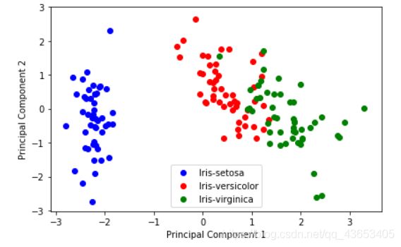
可以发现效果好了些
实际应用中可以直接调库
#小例子
from sklearn.decomposition import PCA
import numpy as np
from sklearn.preprocessing import StandardScaler

x=np.array([[10001,2,55], [16020,4,11], [12008,6,33], [13131,8,22]])

# feature normalization (feature scaling)
X_scaler = StandardScaler()
x = X_scaler.fit_transform(x)

# PCA
pca = PCA(n_components=0.9)# 保证降维后的数据保持90%的信息
pca.fit(x)
pca.transform(x)
总结一下降维过程碰到的Error和解决方法:
- 出现 ‘DataFrame’ object has no attribute ‘ix’
原因:新库不支持df.ix,要改成df.iloc才能正常运行,如将
X = df.ix[:,0:4].values
改为
X = df.iloc[:,0:4].values
问题解决。