CS231n-assignment1-two-Layer Neural Network

In[1]:

import numpy as np
import matplotlib.pyplot as plt

from cs231n.classifiers.neural_net import TwoLayerNet

from __future__ import print_function

#%matplotlib inline
plt.rcParams['figure.figsize'] = (10.0, 8.0) # set default size of plots
plt.rcParams['image.interpolation'] = 'nearest'
plt.rcParams['image.cmap'] = 'gray'

%load_ext autoreload
%autoreload 2

def rel_error(x, y):
    """ returns relative error """
    return np.max(np.abs(x - y) / (np.maximum(1e-8, np.abs(x) + np.abs(y))))

创建一个小的网和一些小数据来检查您的实现。
注意，我们为可重复实验设置了随机种子
ln[2]:

input_size = 4
hidden_size = 10
num_classes = 3
num_inputs = 5

def init_toy_model():
    np.random.seed(0)
    return TwoLayerNet(input_size, hidden_size, num_classes, std=1e-1)

def init_toy_data():
    np.random.seed(1)
    X = 10 * np.random.randn(num_inputs, input_size)
    y = np.array([0, 1, 2, 2, 1])
    return X, y

net = init_toy_model()
X, y = init_toy_data()

正向传递：

反向传递：

计算score：
完成classifiers/neural.py中的TwoLayerNet.loss填写：

    def loss(self, X, y=None, reg=0.0):
        """
        Compute the loss and gradients for a two layer fully connected neural
        network.

        Inputs:
        - X: Input data of shape (N, D). Each X[i] is a training sample.
        - y: Vector of training labels. y[i] is the label for X[i], and each y[i] is
          an integer in the range 0 <= y[i] < C. This parameter is optional; if it
          is not passed then we only return scores, and if it is passed then we
          instead return the loss and gradients.
        - reg: Regularization strength.

        Returns:
        If y is None, return a matrix scores of shape (N, C) where scores[i, c] is
        the score for class c on input X[i].

        If y is not None, instead return a tuple of:
        - loss: Loss (data loss and regularization loss) for this batch of training
          samples.
        - grads: Dictionary mapping parameter names to gradients of those parameters
          with respect to the loss function; has the same keys as self.params.
        """
        # Unpack variables from the params dictionary
        W1, b1 = self.params['W1'], self.params['b1']
        W2, b2 = self.params['W2'], self.params['b2']
        N, D = X.shape

        # Compute the forward pass
        scores = None
        #############################################################################
        # TODO: Perform the forward pass, computing the class scores for the input. #
        # Store the result in the scores variable, which should be an array of      #
        # shape (N, C).                                                             #
        #############################################################################
        fc1 = X.dot(W1) + b1  # fully connected
        X2 = np.maximum(0, fc1)  # ReLU
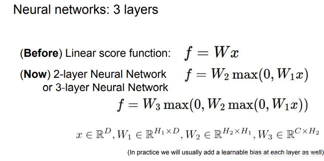
        #2-layer参数表达式
        scores = X2.dot(W2) + b2  # fully connected
        #############################################################################
        #                              END OF YOUR CODE                             #
        #######################################################################3######

        # If the targets are not given then jump out, we're done
        if y is None:
            return scores

        # Compute the loss
        loss = None
        #############################################################################
        # TODO: Finish the forward pass, and compute the loss. This should include  #
        # both the data loss and L2 regularization for W1 and W2. Store the result  #
        # in the variable loss, which should be a scalar. Use the Softmax           #
        # classifier loss.                                                          #
        #############################################################################
        scores -= np.max(scores, axis=1, keepdims=True)  # avoid numeric instability
        scores_exp = np.exp(scores)
        softmax_matrix = scores_exp / np.sum(scores_exp, axis=1, keepdims=True)
        loss = np.sum(-np.log(softmax_matrix[np.arange(N), y]))
        loss /= N
        loss += reg * (np.sum(W2 * W2) + np.sum(W1 * W1))  # regularization
        #############################################################################
        #                              END OF YOUR CODE                             #
        #############################################################################

        # Backward pass: compute gradients
        grads = {}
        #############################################################################
        # TODO: Compute the backward pass, computing the derivatives of the weights #
        # and biases. Store the results in the grads dictionary. For example,       #
        # grads['W1'] should store the gradient on W1, and be a matrix of same size #
        #############################################################################
        softmax_matrix[np.arange(N), y] -= 1
        softmax_matrix /= N
		
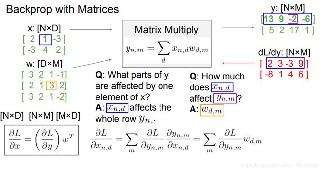
		#开始反向推导
        # W2 gradient
        dW2 = X2.T.dot(softmax_matrix)  # [HxN] * [NxC] = [HxC]

        # b2 gradient
        db2 = softmax_matrix.sum(axis=0)

        # W1 gradient
        dW1 = softmax_matrix.dot(W2.T)  # [NxC] * [CxH] = [NxH]
        dfc1 = dW1 * (fc1 > 0)  # [NxH] . [NxH] = [NxH]
        dW1 = X.T.dot(dfc1)  # [DxN] * [NxH] = [DxH]

        # b1 gradient
        db1 = dfc1.sum(axis=0)

        # regularization gradient
        dW1 += reg * 2 * W1
        dW2 += reg * 2 * W2

        grads = {'W1': dW1, 'b1': db1, 'W2': dW2, 'b2': db2}
        #############################################################################
        #                              END OF YOUR CODE                             #
        #############################################################################

        return loss, grads

ln[3]:

scores = net.loss(X)
print('Your scores:')
print(scores)
print()
print('correct scores:')
correct_scores = np.asarray([
  [-0.81233741, -1.27654624, -0.70335995],
  [-0.17129677, -1.18803311, -0.47310444],
  [-0.51590475, -1.01354314, -0.8504215 ],
  [-0.15419291, -0.48629638, -0.52901952],
  [-0.00618733, -0.12435261, -0.15226949]])
print(correct_scores)
print()

# The difference should be very small. We get < 1e-7
print('Difference between your scores and correct scores:')
print(np.sum(np.abs(scores - correct_scores)))

计算损失(正向)：
与softmax类似，详细见我的上一篇blog
In[4]:

loss, _ = net.loss(X, y, reg=0.05)
correct_loss = 1.30378789133

# should be very small, we get < 1e-12
print('Difference between your loss and correct loss:')
print(np.sum(np.abs(loss - correct_loss)))

计算损失(反向):
ln[5]:

from cs231n.gradient_check import eval_numerical_gradient

loss, grads = net.loss(X, y, reg=0.05)

# these should all be less than 1e-8 or so
for param_name in grads:
    f = lambda W: net.loss(X, y, reg=0.05)[0]
    param_grad_num = eval_numerical_gradient(f, net.params[param_name], verbose=False)
    print('%s max relative error: %e' % (param_name, rel_error(param_grad_num, grads[param_name])))

我们将使用随机梯度下降(SGD)，类似于SVM和Softmax分类器。训练并填写TwoLayerNet函数缺失的部分，以执行测试程序。这应该与用于SVM和Softmax分类器的测试过程非常相似。完成填写TwoLayerNet.predict，因为训练过程定期进行预测，以保持准确性随着时间的推移，训练一旦实现了该方法，运行下面的代码来测试少部分数据的两层网络。你的测试损失应该小于0.2
train函数：

 def train(self, X, y, X_val, y_val,
              learning_rate=1e-3, learning_rate_decay=0.95,
              reg=5e-6, num_iters=100,
              batch_size=200, verbose=False):
        """
        Train this neural network using stochastic gradient descent.

        Inputs:
        - X: A numpy array of shape (N, D) giving training data.
        - y: A numpy array f shape (N,) giving training labels; y[i] = c means that
          X[i] has label c, where 0 <= c < C.
        - X_val: A numpy array of shape (N_val, D) giving validation data.
        - y_val: A numpy array of shape (N_val,) giving validation labels.
        - learning_rate: Scalar giving learning rate for optimization.
        - learning_rate_decay: Scalar giving factor used to decay the learning rate
          after each epoch.
        - reg: Scalar giving regularization strength.
        - num_iters: Number of steps to take when optimizing.
        - batch_size: Number of training examples to use per step.
        - verbose: boolean; if true print progress during optimization.
        """
        num_train = X.shape[0]
        iterations_per_epoch = max(num_train / batch_size, 1)

        # Use SGD to optimize the parameters in self.model
        loss_history = []
        train_acc_history = []
        val_acc_history = []

        for it in range(num_iters):
            X_batch = None
            y_batch = None

            #########################################################################
            # TODO: Create a random minibatch of training data and labels, storing  #
            # them in X_batch and y_batch respectively.                             #
            #########################################################################
            # *****START OF YOUR CODE (DO NOT DELETE/MODIFY THIS LINE)*****

            mask = np.random.choice(num_train, batch_size)
            X_batch = X[mask]
            y_batch = y[mask]

            # *****END OF YOUR CODE (DO NOT DELETE/MODIFY THIS LINE)*****

            # Compute loss and gradients using the current minibatch
            loss, grads = self.loss(X_batch, y=y_batch, reg=reg)
            loss_history.append(loss)

            #########################################################################
            # TODO: Use the gradients in the grads dictionary to update the         #
            # parameters of the network (stored in the dictionary self.params)      #
            # using stochastic gradient descent. You'll need to use the gradients   #
            # stored in the grads dictionary defined above.                         #
            #########################################################################
            # *****START OF YOUR CODE (DO NOT DELETE/MODIFY THIS LINE)*****

            dW1, db1 = grads['W1'], grads['b1']
            dW2, db2 = grads['W2'], grads['b2']
            W1, b1 = self.params['W1'], self.params['b1']
            W2, b2 = self.params['W2'], self.params['b2']
            W1 -= learning_rate * dW1
            b1 -= learning_rate * db1
            W2 -= learning_rate * dW2
            b2 -= learning_rate * db2

            # *****END OF YOUR CODE (DO NOT DELETE/MODIFY THIS LINE)*****

            if verbose and it % 100 == 0:
                print('iteration %d / %d: loss %f' % (it, num_iters, loss))

            # Every epoch, check train and val accuracy and decay learning rate.
            if it % iterations_per_epoch == 0:
                # Check accuracy
                train_acc = (self.predict(X_batch) == y_batch).mean()
                val_acc = (self.predict(X_val) == y_val).mean()
                train_acc_history.append(train_acc)
                val_acc_history.append(val_acc)

                # Decay learning rate
                learning_rate *= learning_rate_decay

        return {
          'loss_history': loss_history,
          'train_acc_history': train_acc_history,
          'val_acc_history': val_acc_history,
        }

预测函数：

    def predict(self, X):
        """
        Use the trained weights of this two-layer network to predict labels for
        data points. For each data point we predict scores for each of the C
        classes, and assign each data point to the class with the highest score.

        Inputs:
        - X: A numpy array of shape (N, D) giving N D-dimensional data points to
          classify.

        Returns:
        - y_pred: A numpy array of shape (N,) giving predicted labels for each of
          the elements of X. For all i, y_pred[i] = c means that X[i] is predicted
          to have class c, where 0 <= c < C.
        """
        y_pred = None

        ###########################################################################
        # TODO: Implement this function; it should be VERY simple!                #
        ###########################################################################
        # *****START OF YOUR CODE (DO NOT DELETE/MODIFY THIS LINE)*****

        scores = self.loss(X)
        y_pred = np.argmax(scores, axis=1)

        # *****END OF YOUR CODE (DO NOT DELETE/MODIFY THIS LINE)*****

        return y_pred

In[6]:

net = init_toy_model()
stats = net.train(X, y, X, y,
            learning_rate=1e-1, reg=5e-6,
            num_iters=100, verbose=False)

print('Final training loss: ', stats['loss_history'][-1])

# plot the loss history
plt.plot(stats['loss_history'])
plt.xlabel('iteration')
plt.ylabel('training loss')
plt.title('Training Loss history')
plt.show()

载入数据:
In[7]:

from cs231n.data_utils import load_CIFAR10

def get_CIFAR10_data(num_training=49000, num_validation=1000, num_test=1000):
    """
    Load the CIFAR-10 dataset from disk and perform preprocessing to prepare
    it for the two-layer neural net classifier. These are the same steps as
    we used for the SVM, but condensed to a single function.  
    """
    # Load the raw CIFAR-10 data
    cifar10_dir = 'assignment1/cs231n/datasets/cifar-10-batches-py'
    
    X_train, y_train, X_test, y_test = load_CIFAR10(cifar10_dir)
        
    # Subsample the data
    mask = list(range(num_training, num_training + num_validation))
    X_val = X_train[mask]
    y_val = y_train[mask]
    mask = list(range(num_training))
    X_train = X_train[mask]
    y_train = y_train[mask]
    mask = list(range(num_test))
    X_test = X_test[mask]
    y_test = y_test[mask]

    # Normalize the data: subtract the mean image
    mean_image = np.mean(X_train, axis=0)
    X_train -= mean_image
    X_val -= mean_image
    X_test -= mean_image

    # Reshape data to rows
    X_train = X_train.reshape(num_training, -1)
    X_val = X_val.reshape(num_validation, -1)
    X_test = X_test.reshape(num_test, -1)

    return X_train, y_train, X_val, y_val, X_test, y_test


# Cleaning up variables to prevent loading data multiple times (which may cause memory issue)
try:
   del X_train, y_train
   del X_test, y_test
   print('Clear previously loaded data.')
except:
   pass

# Invoke the above function to get our data.
X_train, y_train, X_val, y_val, X_test, y_test = get_CIFAR10_data()
print('Train data shape: ', X_train.shape)
print('Train labels shape: ', y_train.shape)
print('Validation data shape: ', X_val.shape)
print('Validation labels shape: ', y_val.shape)
print('Test data shape: ', X_test.shape)
print('Test labels shape: ', y_test.shape)

In[8]:
我们将使用SGD来测试我们的神经网络，调整学习率

input_size = 32 * 32 * 3
hidden_size = 50
num_classes = 10
net = TwoLayerNet(input_size, hidden_size, num_classes)

# Train the network
stats = net.train(X_train, y_train, X_val, y_val,
            num_iters=1000, batch_size=200,
            learning_rate=1e-4, learning_rate_decay=0.95,
            reg=0.25, verbose=True)

# Predict on the validation set
val_acc = (net.predict(X_val) == y_val).mean()
print('Validation accuracy: ', val_acc)

使用我们上面提供的默认参数，您应该在验证集中获得约0.29的验证精度。这不是很好。

了解问题所在的一种策略是在优化过程中在训练和验证集上绘制损失函数和准确性。

另一个策略是将在网络第一层学到的权值可视化。在大多数用视觉数据训练的神经网络中，第一层权重在可视化时通常会显示一些可见的结构。
In[9]:

plt.subplot(2, 1, 1)
plt.plot(stats['loss_history'])
plt.title('Loss history')
plt.xlabel('Iteration')
plt.ylabel('Loss')

plt.subplot(2, 1, 2)
plt.plot(stats['train_acc_history'], label='train')
plt.plot(stats['val_acc_history'], label='val')
plt.title('Classification accuracy history')
plt.xlabel('Epoch')
plt.ylabel('Clasification accuracy')
plt.legend()
plt.show()

In[10]:
可视化W

from cs231n.vis_utils import visualize_grid

# Visualize the weights of the network

def show_net_weights(net):
    W1 = net.params['W1']
    W1 = W1.reshape(32, 32, 3, -1).transpose(3, 0, 1, 2)
    plt.imshow(visualize_grid(W1, padding=3).astype('uint8'))
    plt.gca().axis('off')
    plt.show()

show_net_weights(net)

从上面的可视化图中，我们可以看到损失的减少或多或少是线性的，这似乎表明学习率可能太低了。此外，训练的准确性和验证的准确性之间没有差距，说明我们使用的模型容量较低，我们应该增加它的规模。另一方面，对于一个非常大的模型，我们期望看到更多的过拟合，这将显示出训练和验证精度之间的一个非常大的差距。
调节超参数和发现它们如何影响最终表现的直觉是使用神经网络的很重要的部分，所以我们希望你得到大量的练习。下面，您应该试验各种超参数的不同值，包括隐藏层大小、学习速率、训练数和正则化强度。您也可以考虑调优学习速率衰减，但是使用默认值应该能够获得良好的性能
您的目标应该是在验证集上实现大于48%的分类精度。我们最好在验证集上超过52%。
实验:在这个练习中，您的目标是通过一个完全连接的神经网络在CIFAR-10上获得尽可能好的结果。你可以自由地实现你自己的技术(例如PCA来降低维数，或添加dropout，或向求解器添加功能，等等)。
In[11]:

best_net = None # store the best model into this 
best_val = -1
best_stats = []
#################################################################################
# TODO: Tune hyperparameters using the validation set. Store your best trained  #
# model in best_net.                                                            #
#                                                                               #
# To help debug your network, it may help to use visualizations similar to the  #
# ones we used above; these visualizations will have significant qualitative    #
# differences from the ones we saw above for the poorly tuned network.          #
#                                                                               #
# Tweaking hyperparameters by hand can be fun, but you might find it useful to  #
# write code to sweep through possible combinations of hyperparameters          #
# automatically like we did on the previous exercises.                          #
#################################################################################
# generate random hyperparameters given ranges for each of them
def generate_random_hyperparams(lr_min, lr_max, reg_min, reg_max, h_min, h_max):
    lr = 10**np.random.uniform(lr_min,lr_max)
    reg = 10**np.random.uniform(reg_min,reg_max)
    hidden = np.random.randint(h_min, h_max)
    return lr, reg, hidden

# get random hyperparameters given arrays of potential values
def random_search_hyperparams(lr_values, reg_values, h_values):
    lr = lr_values[np.random.randint(0,len(lr_values))]
    reg = reg_values[np.random.randint(0,len(reg_values))]
    hidden = h_values[np.random.randint(0,len(h_values))]
    return lr, reg, hidden

input_size = 32 * 32 * 3
num_classes = 10

# Set a seed for results reproduction
np.random.seed(0)

# Use of random search for hyperparameter search
for i in range(20):
    ## Strategy to find the best hyperparameters over 52% on the validation set
    # Use generate_random function given some interval with 500 iterations
    #lr, reg, hidden_size = generate_random_hyperparams(-6, -3, -5, 5, 20, 3000)
    #lr, reg, hidden_size = generate_random_hyperparams(-4, -2, -2, 2, 20, 3000)
    #lr, reg, hidden_size = generate_random_hyperparams(-4, -3, -1, 0, 10, 300)
    
    # According to the previous results, reduce the exploration by selecting set of fixed ranges
    # use this ranges in the random search function to explore random combinations
    #lr, reg, hidden_size = random_search_hyperparams([0.001, 0.002, 0.003], [0.1, 0.2, 0.3, 0.4, 0.5], [10, 50, 100, 150, 200])
    #lr, reg, hidden_size = random_search_hyperparams([0.001], [0.1, 0.15, 0.2, 0.3], [10, 20, 30, 40 ,50, 80, 100, 150 , 200])    
    
    # Given a set of potential values, increase the number of iterations
    lr, reg, hidden_size = random_search_hyperparams([0.001], [0.05, 0.1, 0.15], [50, 80, 100, 120, 150, 180, 200])
    
    # Create a two-layer network
    net = TwoLayerNet(input_size, hidden_size, num_classes)
    
    # Train the network
    stats = net.train(X_train, y_train, X_val, y_val,
                num_iters=2000, batch_size=200,
                learning_rate=lr, learning_rate_decay=0.95,
                reg=reg, verbose=False)

    # Predict on the training set
    train_accuracy = (net.predict(X_train) == y_train).mean()
    
    # Predict on the validation set
    val_accuracy = (net.predict(X_val) == y_val).mean()
    
    # Save best values
    if val_accuracy > best_val:
        best_val = val_accuracy
        best_net = net
        best_stats = stats
    
    # Print results
    print('lr %e reg %e hid %d  train accuracy: %f val accuracy: %f' % (
                lr, reg, hidden_size, train_accuracy, val_accuracy))
print('best validation accuracy achieved: %f' % best_val)
#################################################################################
#                               END OF YOUR CODE                                #
#################################################################################

绘制损失函数验证损失率
In[12]:

plt.subplot(2, 1, 1)
plt.plot(best_stats['loss_history'])
plt.title('Loss history')
plt.xlabel('Iteration')
plt.ylabel('Loss')

plt.subplot(2, 1, 2)
plt.plot(best_stats['train_acc_history'], label='train')
plt.plot(best_stats['val_acc_history'], label='val')
plt.title('Classification accuracy history')
plt.xlabel('Epoch')
plt.ylabel('Clasification accuracy')
plt.legend()
plt.show()

In[13]:
最佳W可视化

show_net_weights(best_net)

In[14]:
当你完成了实验，你应该在测试集中评估你最终训练的网络;应该在48%以上。
测试：

test_acc = (best_net.predict(X_test) == y_test).mean()
print('Test accuracy: ', test_acc)

内联的问题

现在您已经训练了一个神经网络分类器，您可能会发现您的测试精度远远低于训练精度。我们怎样才能缩小这一差距呢?

1.训练更大的数据集。
2.增加正则化强度。
在更大的数据集上训练可以防止过拟合。例如，在CIFAR数据集中，添加具有不同变体的每个类的更多样本将允许模型更好地泛化。然而，如果我们添加的数据是有不好的或与我们已有的数据类似，那么它就不会有太大的帮助。
增加正则化强度避免了过拟合的问题，因为它降低了模型的复杂性，因此使用正则化可以训练复杂的模型。