【基于Python的概率论与数理统计实验】实验1_抛硬币实验的模拟
【基于Python的概率论与数理统计实验】实验1_抛硬币实验的模拟
一、实验目的
1.通过抛硬币实验来验证频率具有稳定性。
2.学会使用Python作图。
二、实验要求
1.复习大数定律。
2.画图显示运行结果。
三、实验内容
利用Python编写程序,以产生一系列0和1的随机数,模拟抛硬币实验。验证抛一枚质地均匀的硬币,正面向上事件频率的稳定值为0.5。
四、实验步骤
(1)生成0和1的随机数序列,将其放入列表count中,也可用函数表示。
(2)统计0和1出现的次数,将其放入a中。a[0]、a[1]分别表示0和1出现的次数。
(3)画图展示每次实验正面向上事件的频率。
# 方法1:使用Counter函数进行计数
from collections import Counter
import matplotlib.pyplot as plt
import random
from time import perf_counter

start=perf_counter()       #计时开始
times = 10000
count = []  # 将每次随机出现的数字放入列表
for i in range(1, times+1):
    y = random.randint(0, 1)
    count.append(y)
#统计0和1出现的次数,计算频率,1表示正面向上
#直接统计每个数字出现的次数,a[0],a[1]分别表示0和1出现的次数
a = Counter(count)
f1=a[1]
print(f1/times)

#画图展示每次实验正面向上出现的频率
f = []  #存储朝上的频率
indices=[]
#i表示做的试验次数
for i in range(1,times+1):
    heads = 0   #做i次试验正面向上出现的次数
    for j in range(i):
        if count[j]==1:
            heads+=1
    f.append(heads/i)   #计算频率
    indices.append(i)   #第i次试验

#作图
plt.figure(figsize=(18, 8))
plt.rcParams['font.sans-serif'] = 'SimHei'  # 设置中文显示
plt.rcParams['axes.unicode_minus'] = False
plt.xlim(0, times)
plt.ylim(0, 1)
plt.plot(indices,f)
plt.plot([0,times],[0.5,0.5],color='r')
plt.text(0,0.5,'0.5',color='r',fontsize=16)
plt.xlabel('试验次数')
plt.ylabel('频率')
plt.show()
print("运行时间是: {:.5f}s".format(perf_counter()-start))
0.5026
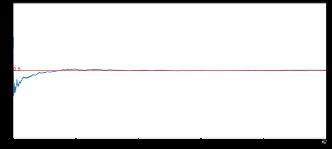
运行时间是: 4.40956s
结论:当实验次数足够大时,正面向上事件的频率稳定在0.5附近。
# 方法2:不使用Counter函数进行计数
import matplotlib.pyplot as plt
import random
from time import perf_counter

start=perf_counter()       #计时开始
times = 10000
count = []  # 将每次随机出现的数字放入列表
for i in range(1, times+1):
    y = random.randint(0, 1)
    count.append(y)
#统计0和1出现的次数,计算频率,1表示正面向上
s1=0
s2=0
for k in count:
    if k ==0:
        s1+= 1
    else:
        s2+=1
f1=s2
print(f1/times)
#画图展示每次试验正面向上出现的频率

f = []  #存储朝上的频率
indices=[]
#i表示做的试验次数
for i in range(1,times+1):
    heads = 0 #做i次实验正面向上事件的次数
    for j in range(i):
        if count[j]==1:
            heads+=1
    f.append(heads/i) #计算频率
    indices.append(i)   #第i次试验

#作图
plt.figure(figsize=(18, 8))
plt.rcParams['font.sans-serif'] = 'SimHei'  # 设置中文显示
plt.rcParams['axes.unicode_minus'] = False
plt.xlim(0, times)
plt.ylim(0, 1)
plt.plot(indices,f)
plt.plot([0,times],[0.5,0.5],color='r')
plt.text(0,0.5,'0.5',color='r',fontsize=16)
plt.xlabel('试验次数')
plt.ylabel('频率')
plt.show()
print("运行时间是: {:.5f}s".format(perf_counter()-start))
0.5011

运行时间是: 4.40306s
# 方法3:自定义函数
import matplotlib.pyplot as plt
import random
from time import perf_counter

#返回0或者1
def r():
    s=random.randint(0,1)
    return s

start=perf_counter()       #计时开始
times=5000
indices=[]
f = []   #存储朝上的频率
for i in range(1,times+1):
    heads = 0  #做i次实验正面向上事件次数
    for j in range(i):
        if r() == 1:
            heads+=1
    f.append(heads/i)
    indices.append(i)
print(heads/times)

#作图
plt.figure(figsize=(18, 8))
plt.rcParams['font.sans-serif'] = 'SimHei'  # 设置中文显示
plt.rcParams['axes.unicode_minus'] = False
plt.xlim(0, times)
plt.ylim(0, 1)
plt.plot(indices,f)
plt.plot([0,times],[0.5,0.5],color='r')
plt.text(0,0.5,'0.5',color='r',fontsize=16)
plt.xlabel('试验次数')
plt.ylabel('频率')
plt.show()
print("运行时间是: {:.5f}s".format(perf_counter()-start))
0.5034
运行时间是: 9.23432s
# 方法4(向量化思维)
import numpy as np
import matplotlib.pyplot as plt
from time import perf_counter

start=perf_counter()       #计时开始
coin=[0,1]     #1-正面,0-反面
sim=10000      #模拟次数
t=np.zeros(sim) #存储每次抽样的结果
f=np.zeros(sim) #存储朝上的频率
for i in range(sim):
    a=np.random.choice(coin,1)    #抽样
    t[i]=a==1
    f[i]=np.mean(t[0:i+1])
print(np.mean(t))
indices=np.arange(1,sim+1)

#作图
plt.figure(figsize=(18, 8))
plt.rcParams['font.sans-serif'] = 'SimHei'  # 设置中文显示
plt.rcParams['axes.unicode_minus'] = False
plt.xlim(0, sim)
plt.ylim(0, 1)
plt.plot(indices,f)
plt.plot([0,sim],[0.5,0.5],color='r')
plt.text(0,0.5,'0.5',color='r',fontsize=16)
plt.xlabel('试验次数')
plt.ylabel('频率')
plt.show()
print("运行时间是: {:.5f}s".format(perf_counter()-start))
0.5087
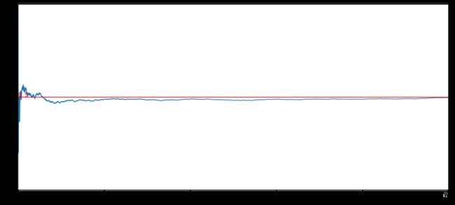
运行时间是: 0.31413s