Modern Robotics逆运动学数值解法及SVD算法

Modern Robotics运动学数值解法及SVD算法

前言

这半个月的业余时间研究了机器人逆运动学的解析解法和迭代数值解法，并用程序实现。由于解析法只适合于特定结构的机器人，不具有通用性，因此这里不讨论解析解，只讨论迭代数值解法。本文相关的程序及研究素材都可以从github下载–链接 。

数值逆运动学

机器人逆运动学的解析解虽然很优美，但是有时候获得解析解很困难，甚至以人类的智慧无法求得解析解，这时候就可以用迭代数值解法。即使存在解析解，数值解法也经常用来提高解的精度。例如PUMA类型的机器人，最后三个轴由于机械制造和装配误差，实际上可能没有相交于一点，肩关节的轴线也可能不垂直。这种情况下，不必抛弃任何可用的解析解，这些解可以作为迭代数值解法的初始值。

求解非线性方程的根有多种迭代方法，我们将使用一种非线性求根的基本方法，牛顿拉普森法。此外，在不存在精确解的情况下，我们需要寻找最接近的近似解，这就需要优化方法。因此，我们现在讨论非线性求根的牛顿拉普森方法，以及优化的一阶必要条件。

牛顿-拉普森方法

对于一个给定的可微函数$g:\mathbb{R}\to \mathbb{R}$, 假设${\theta }_0$是一个猜测的初值，求方程$g(\theta )=0$的数值解。对$g(\theta )=0$在${\theta }_0$处进行一阶截断，其泰勒展开式为
$$g(\theta )=g({\theta }_0)+\frac{\partial g}{\partial \theta }({\theta }_0)(\theta -{\theta }_0)+\text{higher-order terms}$$
只保留一阶项，设$g(\theta )=0$，那么可求得$\theta$为
$$\theta ={\theta }_0-{\left(\frac{\partial g}{\partial \theta }({\theta }^0)\right)}^{-1}g({\theta }^0)$$
使用$\theta$值作为新的猜测的解，重复上面的计算，就得到下面的迭代式
$${\theta }^{k+1}={\theta }^k-{\left(\frac{\partial g}{\partial \theta }({\theta }^k)\right)}^{-1}g({\theta }^0).$$
重复上式的迭代直到某些判断满足，例如对于用户预先设定的值$ϵ$,满足$g({\theta }^k)-g({\theta }^{k+1}|/|g({\theta }^k|\le ϵ$。

当$g$是多维的时候，也使用同样的公式。例如$g:{\mathbb{R}}^n\to {\mathbb{R}}^n$,
$$\frac{\partial \theta }{\partial \theta }(\theta )=\left[\begin{array}{ccc}\frac{\partial g_1}{\partial {\theta }_1}(\theta )& \dots & \frac{\partial g_1}{\partial {\theta }_n}(\theta )\\ ⋮& \ddots ⋮& \\ \frac{\partial g_n}{\partial {\theta }_1}(\theta )& \dots & \frac{\partial g_n}{\partial {\theta }_n}(\theta )\end{array}\right]\in {\mathbb{R}}^{n\times n}$$
下面我们讨论该矩阵不可逆的情形。

数值逆运动学算法

假设我们用一个坐标向量$x$表示末端坐标系，由正运动学$x=f(\theta )$控制, 这是一个非线性向量方程，映射了$n$个关节坐标到$m$个末端坐标。假设$f:{\mathbb{R}}^n\to {\mathbb{R}}^m$可导，设$x_d$是期望的末端坐标。那么$g(\theta )$的牛顿拉普森方法定义为$g(\theta )=x_d-f(\theta )$, 目标是寻找关节坐标$\theta$使得
$$g({\theta }_d)=x_d-f({\theta }_d).$$
给定初始值${\theta }_0$ “接近”于一个解${\theta }_d$, 所谓“接近”只是认为其接近，不一定是接近，但在迭代过程中会逐渐接近，如图所示。运动学方程可写成泰勒展开式
$$x_d=f({\theta }_d)=f({\theta }^0)+\underset{J({\theta }^0)}{\frac{\partial f}{\partial \theta }|{\theta }^0}\underset{\Delta \theta }{({\theta }_d-{\theta }^0)}+\text{h.o.t}\text{\hspace{1em}(6.3)}$$
这里$J({\theta }^0)\in {\mathbb{R}}^{m\times n}$是在${\theta }^0$处的雅可比坐标。一阶截断泰勒展开式，我们得到上式的近似方程
$$J({\theta }^0)\Delta \theta =x_d-f({\theta }^0).\text{\hspace{1em}(6.4)}$$
假设$J({\theta }^0)$是方阵并且可导，我们可以得到

$$\Delta \theta =J^{-1}({\theta }^0)(x_d-f({\theta }^0)).\text{\hspace{1em}(6.5)}$$
如果正运动学方程是关于$\theta$的线性方程，那么方程（6.3）的高阶项是0，新的猜测值${\theta }^1={\theta }^0+\Delta \theta$确实满足$x_d=f({\theta }^1)$. 如果正运动学不是关于$\theta$是线性的，这是常见的情形，这性的猜测值${\theta }^1$仍然是比${\theta }^0$更接近真实解的，这个过程不断重复，就会产生一个序列$\{{\theta }^0,{\theta }^1,{\theta }^2,\dots \}$收敛于 ${\theta }_d$(如图所示).

**图示说明：**牛顿拉普森法求解非线性方程的根。在第一步，斜率$-\frac{\partial f}{\partial \theta }$在点(${\theta }^0,x_d-f({\theta }^0)$)计算得到。第二步，斜率在(${\theta }^1,x_d-f({\theta }^1)$)处计算得到，最后这样的过程会收敛于${\theta }_d$。 注意到，初始值在函数$x_d-f(\theta )$的极点左边时，很可能导致收敛于另外一个根，如果初始值在极点或靠近极点时，会导致$\Delta \theta$的初始值很大，迭代过程可能根本不收敛。

像上图显示那样，如果你运动学存在多解，迭代过程倾向于收敛到“最靠近”初始值${\theta }^0$的根。你可以认为每个根有自己的吸引力区域，如果初始值没有落在这些吸引力区域(例如初始值收敛于一个根的效率很低)，迭代过程可能是不收敛的。

实际应用中，由于计算效率的原因，求解方程(6.4)通常不直接计算逆矩阵$J^{-1}({\theta }^0)$。 有更高效的方法求解线性方程组$Ax=b$的方法。例如，对于可逆矩阵$A$, 进行LU分解来求解$x$计算量更少。例如在MATLAB里，下面命令

x=A\b

求解$Ax=b$时不计算$A^{-1}$。

如果由于不是方阵或奇异，$J$不可逆，那么方程（6.5）的$J^{-1}$不存在。通过使用广义逆(Moore-Penrose pseudoinverse) $J^{†}$替换方程(6.5)的$J^{-1}$， 方程(6.4)仍然可以求解$\Delta \theta$（或者说求近似解）。对于形式为$Jy=z$的方程，$J\in {\mathbb{R}}^{m\times n},y\in {\mathbb{R}}^n,z\in {\mathbb{R}}^m$ ，它的解为
$$y\ast =J^{†}z$$
需要分两种情况讨论得到的解

• 该解$y\ast$确实满足$Jy\ast =z$， 并且任意解$y$满足$Jy=z$，并且$||y\ast ||\le ||y||$。 也就是说，在所有的解中，$y\ast$的2范数最小。机器人的关节数n大于末端坐标m时，$Jy=z$有无穷多个解，这时称$J$是“胖”的。
• 如果没有$y$满足$Jy=z$， 那么$y\ast$是误差的2范数最小的解，即对于任意$y\in {\mathbb{R}}^n,||Jy\ast -z||\le ||Jy-z||$ . 这种情形对应于rank $J\le m$。例如机器人的关节数小于末端坐标数m（"瘦"的雅可比$J$）或者出现奇异。

有很多计算伪逆（广义逆）的方法，在matlab里是

y=pinv(J)*z

当$J$是满秩（rank $m$，$n>m$ 或秩 rank $n$, $n<m$）, 例如根没有在奇异处，伪逆可以按下式计算

$J^{†}=J^T(J{J}^T{)}^{-1}$ 如果$J$是胖的, $n>m$ (称为右逆，因为$J{J}^{†}=I$)

$J^{†}=(J^{T}J{)}^{-1}J$ 如果$J$是瘦的，$n<m$ (称为左逆，因为$J^{†}J=I$).

使用伪逆计算雅可比的逆，方程(6.5)可以写成
$$\Delta \theta =J^{†}({\theta }^0)(x_d-f({\theta }^0)).\text{\hspace{1em}(6.6)}$$
如果$\text{rank }(J)<m$ ，那么方程(6.6)的解$\Delta \theta$可能不满足方程(6.4), 但是从最小方差角度看，这是尽可能满足条件的解。如果$n>m$ ，该解是满足方程(6.4)的关节变量改变最小的解(从2范数角度看)。

在牛顿-拉普森迭代算法中应用方程(6.6)求解${\theta }_d$分为两步

(1) 初始化：给定$x_d\in {\mathbb{R}}^m$ 以及初始${\theta }^0\in {\mathbb{R}}^n$, 令$i=0$。

(2)设 $e=x_d-f({\theta }^i)$. 当对于某个较小的$ϵ$，当$||e||>ϵ$:

• 设置 ${\theta }^{i+1}={\theta }^i+J^{†}({\theta }^I)e$
• 增加 $i$.

适当修改该算法，就可以处理机器人逆运动学问题。机器人末端构型用$T_{sd}\in SE(3)$表示, 替换坐标矢量$x_d$, 坐标雅可比$J$用末端的物体雅可比$J_b\in {\mathbb{R}}^{6\times n}$替换. 但是，向量$e=x_d-f({\theta }^i)$， 表示当前猜测值到末端期望构型的方向(通过正运动学计算)，不能简单地用$T_{sd}-T_{sb}({\theta }^i)$代替。$J_b$的伪逆需要对在物体坐标系表示的旋量${\mathcal{V}}_b\in {\mathbb{R}}^6$进行变换. 为了正确类比，我们把$e=x_d-f({\theta }^i)$看成是一个速度矢量，如果经过一个单位时间，将会产生从$f({\theta }^i)$向$x_d$的运动。相似地，我们应该寻找一个物体坐标系旋量${\mathcal{V}}_b$, 经过单位时间，将会产生一个从$T_{sb}({\theta }^i)$向期望构型$T_{sd}$的运动。

为了寻找这个${\mathcal{V}}_b$， 我们首先计算期望构型在当前物体坐标系的表达
$$T_{bd}({\theta }^i)=T_{sb}^{-1}({\theta }^i)T_{sd}=T_{bs}({\theta }^i)T_{sd}.$$
然后${\mathcal{V}}_b$通过矩阵对数计算
$$[{\mathcal{V}}_b]=\text{log}{T}_{bd}({\theta }^i)$$
这样可以得到以下的逆运动学算法，类似于前面的坐标向量算法：

(1)初始化：给定$T_{sd}$ 和初始值${\theta }^0\in {\mathbb{R}}^n$, 设置$i=0$.

(2)设置$[{\mathcal{V}}_b]=\text{log}(T_{sb}^{-1}({\theta }^i))$, 对给定的误差${ϵ}_w,{ϵ}_v$, 当$||\omega_b||>\epsilon_{\omega} $ 或者$||v_b||>{ϵ}_v$:

• 设置 ${\theta }^{i+1}={\theta }^i+J_b^{†}({\theta }^i){\mathcal{V}}_b$.
• 增加 $i$.

应用空间雅可比$J_s(\theta )$和空间旋量${\mathcal{V}}_s=[{\text{Ad}}_{T_{sb}}]{\mathcal{V}}_b$, 可以推导在固定坐标系的等效形式。

为了数值逆运动学方法收敛，初始值${\theta }^0$需要高效地收敛于${\theta }_d$. 从机器人初始构型开始，就可以满足条件。在初始位置末端的真实构型以及关节角度都是已知的，同时保证末端位置$T_{sd}$在逆运动学计算过程中是缓慢变化的。

补充 ：

以上的分析或许有人觉得有点难理解，例如$T_{bd}$的物理意义是啥？是在哪两个坐标系或矢量的变换？下面结合这个图分析一下，或许有助于理解。

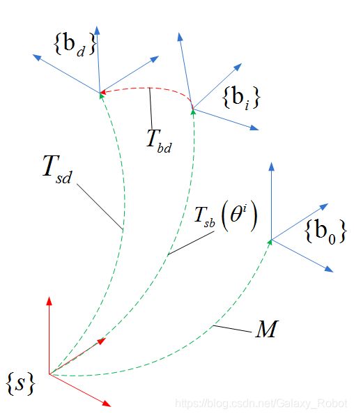
我们知道，一个齐次矩阵，在不同场合可以有三种不同的含义，（1）它是坐标系的描述，或者说构型，例如$T_{sd}$表示坐标系$\{b_d\}$在坐标系$\{s\}$中的描述，或者说坐标系$\{b_d\}$的构型。（2）它是变换映射。例如$T_{sd}$可以看成是把在坐标系$\{b_d\}$表示的物理量映射到在坐标系$\{s\}$中表示。（3）它是一个变换算子，或者说刚体运动。例如$T_{sd}$可以看成是把坐标系$\{s\}$变换的坐标系$\{b_d\}$的变换算子，或者说$\{s\}$运动到$\{b_d\}$所做的刚体运动。在我们的以上的迭代算法中，我们应该把$M,T_{sb}({\theta }^i),T_{sd}$理解为第一种含义，即坐标系的描述（或构型），把$T_{bd}$理解为第三种含义，即变换算子（或者说刚体运动）。因此，机器人末端$\{b\}$的位姿（构型）初始状态在$\{b_0\}$处，$M$表示机器人末端在坐标系$\{s\}$中的描述，在任意迭代步中，机器人末端$\{b\}$运动到 $\{b_i\}$, $T_{sb}({\theta }^i)$表示此时机器人末端$\{b_i\}$在坐标系$\{s\}$中的描述，这时末端当前位姿（构型）$T_{sb}({\theta }^i)$与期望位姿（构型）$T_{sd}$存在一个"差值" , 与$x_d-f({\theta }^i)$类比. 这个“差值”$T_{bd}$与向量（或者标量）$x_d-f({\theta }^i)$不同，该"差值"是一个变换算子，即刚体运动，表示末端从当前位姿$T_{sb}({\theta }^i)$ （变换）运动到期望位姿$T_{sd}$所需做的（变换算子）刚体运动。那么这个关系可以表示为
$$T_{bd}{T}_{sb}({\theta }^i)=T_{sd}$$
因此有
$$T_{bd}=T_{bd}({\theta }^i)=T_{sb}({\theta }^i{)}^{-1}{T}_{sd}$$
那么这个刚体运动是一个螺旋运动, 指数坐标为$V_b$，它是$T_{bd}$的对数。如图所示，当然$T_{bd}$也可以理解为前面所说的，期望构型在当前物体坐标系的表达。里面包含两个分量，角度位移$w_b$和线位移$v_b$ 。若对给定的误差${ϵ}_w,{ϵ}_v$, 当$||\omega_b||\le \epsilon_{\omega} $ 且$||v_b||\le {ϵ}_v$，那说明当前位姿与期望位姿非常接近，所需做的刚体运动非常小了。当小于给定误差，这时迭代停止，对应的${\theta }^i$即为所需的解。因此有前面的逆运动学算法。

奇异值（SVD）分解算法

前面提到的$J^{†}=J^T(J{J}^T{)}^{-1}$ 或$J^{†}=(J^{T}J{)}^{-1}J$ 计算伪逆，都是要求解逆矩阵的。这里介绍一种应用广泛的方法–奇异值分解(SVD, Singular Value Decomposition ) ，求伪逆矩阵。

在许多情况下，高斯消去法和LU分解法都不能给出满意的结果。有一套非常有用的技术，用来该处理不论是奇异还是数值上非常接近奇异的方程组或矩阵。该方法称为奇异值值分解（SVD）。该方法会精确地告诉我们什么情况属于该类问题。某些情况下，SVD不仅可以判断该问题，还可以求解它，提供一个有用的数值解，尽管这个解不一定是我们想要的。SVD也可以用来求解多数的最小二乘问题。

SVD技术基于下面的线性代数定理。任意$M\times N$的矩阵$A$, 其行数$M$大于或等于列数$N$， 可以写成一个$M\times N$的列正交矩阵$U$， 一个$N\times N$的元素均为正数或零（奇异值）的对角阵$W$, 以及一个$N\times N$正交阵$V$的转置矩阵的乘积形式，如下所示
$$\left(\mathbf{A}\right)=\left(\mathbf{U}\right)\left(\begin{array}{cccc}{w}_0& & & \\ & w_1& & \\ & & \dots & \\ & & \dots & \\ & & & w_{N-1}\end{array}\right)\left({\mathbf{V}}^T\right)\text{\hspace{1em}(1.1)}$$

矩阵$\mathbf{U}$ 和$\mathbf{V}$都是正交的，他们的列是正交标准化的
$$\sum _{i=0}^{M-1}{U}_{ik}{U}_{in}={\delta }_{kn},0\le k\le N-1,0\le n\le N-1\text{\hspace{1em}(1.2)}$$

$$\sum _{j=0}^{N-1}{V}_{ik}{V}_{jn}={\delta }_{kn},0\le k\le N-1,0\le n\le N-1\text{\hspace{1em}(1.3)}$$

或者表示成
$$({\mathbf{U}}^T)(\mathbf{U})=({\mathbf{V}}^T)(\mathbf{V})=(1)\text{\hspace{1em}(1.4)}$$
由于$\mathbf{V}$是方阵，所以它也是行正交标准化的，$\mathbf{V}\cdot {\mathbf{V}}^T=1$.

当$M<N$时，SVD分解也可以执行。这种情况中，奇异值$w_j,j=M,...,N-1$都为零，并且$\mathbf{U}$的列也都为零，这时，仅当$k,n\le M-1$时，(1.2)式成立。

不管矩阵是否奇异，(1.1)式的分解总是可以完成的，而且这个分解几乎是唯一的。也就是说，其分解形式唯一到：（i）对$\mathbf{U}$的列，$\mathbf{W}$的元素和$\mathbf{V}$的列能进行相同的置换；（ii）形成$\mathbf{U}$和$\mathbf{V}$的任意列的线性组合， 其在$\mathbf{W}$中对应的元素查号完全相同。对于$M<N$的情况，这种自由置换的重要结论是，分解的数值算法对$w_j,j=M,...,N-1$要求返回非零，而这$N-M$个零奇异值应分散所有$j=0,1,...,M-1$上。

SVD分解完成之后，我们利用正交矩阵$\mathbf{U}，V$的逆是其转置矩阵，对角阵的逆是其非零元素取倒数。那么可以计算得到矩阵A的伪逆为
$${\mathbf{A}}^{†}=\mathbf{V}\cdot {\mathbf{W}}^{-1}{\mathbf{U}}^T\text{\hspace{1em}(1.5)}$$
关于SVD理论在很多参考书及文献有广泛而深入的探讨，这里不再累赘。

基于SVD分解计算伪逆矩阵（C语言）

下面给出对任意矩阵进行SVD分解以及求伪逆的C程序，SVD分解算法参考《Numerical recipes ,The Art of Scientific Computing, Third Edition 》。主要包括以下几个函数

• void MatrixMult(const double *a, int m, int n, const double *b, int l, double *c);计算任意阶矩阵乘法。
• void MatrixT(double *a, int m, int n, double *b);计算任意阶矩阵的转置。
• int svdcmp(double *a, int m, int n,double tol, double *w, double *v);计算任意阶矩阵SVD分解。
• int MatrixPinv(const double *a, int m, int n, double tol, double *b);基于SVD分解计算任意阶矩阵的伪逆。

下面给出这几个函数的c语言实现代码，代码不断更新迭代，完整的最新源码参见github–链接

头文件声明

/**
 * @brief			Description: Algorithm module of robotics, according to the
 *					book[modern robotics : mechanics, planning, and control].
 * @file:			RobotAlgorithmModule.h
 * @author:			Brian
 * @date:			2019/03/01 12:23
 * Copyright(c) 	2019 Brian. All rights reserved.
 *					  
 * Contact 			https://blog.csdn.net/Galaxy_Robot
 * @note:     
 * @warning: 		
*/

#ifndef SVDPINV_H_
#define SVDPINV_H_
#ifdef __cplusplus
extern "C" {
#endif
  
	/**
	*@brief			Computes Matrix transpose.
	*@param[in]		a			a matrix.
	*@param[in]		m			rows of matrix a.
	*@param[in]		n			columns of matrix a.
	*@param[out]	b			transpose of matrix a.
	*@note:
	*@waring:
	*/
	void MatrixT(double *a, int m, int n, double *b);

	/**
	*@brief			Computes matrix multiply.
	*@param[in]		a		First matrix.
	*@param[in]		m		rows of matrix a.
	*@param[in]		n		columns of matrix b.
	*@param[in]		b		Second matrix.
	*@param[in]		l		columns of matrix b.
	*@param[out]	c		result of a*b.
	*@note:
	*@waring:
	*/
	void MatrixMult(const double *a, int m, int n, const double *b, int l, double *c);
  
	/**
	*@brief			Given the matrix a,this routine computes its singular value decomposition.
	*@param[in/out]	a		input matrix a or output matrix u.
	*@param[in]		m		number of rows of matrix a.
	*@param[in]		n		number of columns of matrix a.
	*@param[in]		tol		any	singular values less than a tolerance are treated as zero.
	*@param[out]	w		output vector w.
	*@param[out]	v		output matrix v.
	*@return        No return value.
	*@note:			input a must be a  m rows and n columns matrix,w is n-vector,v is a n rows and n columns matrix. 
	*@waring:
	*/
	int svdcmp(double *a, int m, int n,double tol, double *w, double *v);
  
	/**
	*@brief			Computes Moore-Penrose pseudoinverse by  Singular Value Decomposition (SVD) algorithm.
	*@param[in]		a			an arbitrary order matrix.
	*@param[in]		m			rows.
	*@param[in]		n			columns.
	*@param[in]		tol			any	singular values less than a tolerance are treated as zero.
	*@param[out]	b			Moore-Penrose pseudoinverse of matrix a.
	*@return        0:success,Nonzero:failure.
	*@retval		0			success.
	*@retval		1			failure when use malloc to allocate memory.
	*@note:
	*@waring:
	*/
	int MatrixPinv(const double *a, int m, int n, double tol, double *b);
  
#ifdef __cplusplus
}
#endif

#endif//SVDPINV_H_

实现文件

/**
 * @brief			Description: Algorithm module of robotics, according to the
 *					book[modern robotics : mechanics, planning, and control].
 * @file:			RobotAlgorithmModule.c
 * @author:			Brian
 * @date:			2019/03/01 12:23
 * Copyright(c) 	2019 Brian. All rights reserved.
 *					  
 * Contact 			https://blog.csdn.net/Galaxy_Robot
 * @note:     
 * @warning: 		
*/
#include "RobotAlgorithmModule.h"
#include 
#include 
#include 
#include 
#define SIGN(a,b) ((b) >= 0.0 ? fabs(a) : -fabs(a))
#define MAX(a,b) (a>b?a:b)
#define MIN(a,b) (a

/**
*@brief			Computes (a^2+b^2)^(1/2),
*@param[in]		a
*@param[in]		b
*@note:
*@waring:
*/
double pythag(const double a, const double b)
{
	double absa, absb;
	absa = fabs(a);
	absb = fabs(b);
	if (absa > absb) return absa*sqrt(1.0 + (absb / absa)*(absb / absa));
	else return (absb == 0.0 ? 0.0 : absb*sqrt(1.0 + (absa / absb)*(absa / absb)));

}
/**
*@brief			Given the matrix a,this routine computes its singular value decomposition.
*@param[in/out]	a		input matrix a or output matrix u.
*@param[in]		m		number of rows of matrix a.
*@param[in]		n		number of columns of matrix a.
*@param[in]		tol		any	singular values less than a tolerance are treated as zero.
*@param[out]	w		output vector w.
*@param[out]	v		output matrix v.	
*@return        No return value.
*@note:			input a must be a  m rows and n columns matrix,w is n-vector,v is a n rows and n columns matrix.
*@waring:
*/
int svdcmp(double *a, int m, int n, double tol, double *w, double *v)
{

	int flag, i, its, j, jj, k, l, nm;
	double anorm, c, f, g, h, s, scale, x, y, z;
	double *rv1 = (double *)malloc(n * sizeof(double));
	if (rv1==NULL)
	{
		return 1;
	}
	g = scale = anorm = 0.0;
	for (i=0;i<n;i++)//Householder reduction to bidiagonal form.
	{
		l = i + 2;
		rv1[i] = scale*g;
		g = s = scale = 0.0;
		if (i<m)
		{
			for (k = i; k < m; k++)scale += fabs(a[k*n + i]);
			if (scale!=0.0)
			{
				for (k = i; k < m;k++)
				{
					a[k*n + i] /= scale;
					s += a[k*n + i] * a[k*n + i];
				}
				f = a[i*n + i];
				g = -SIGN(sqrt(s), f);
				h = f*g - s;
				a[i*n + i] = f - g;
				for (j=l-1;j<n;j++)
				{
					for (s = 0.0, k = i; k < m;k++)
					{
						s += a[k*n + i] * a[k*n + j];
					}
					f = s / h;
					for (k = i; k < m;k++)
					{
						a[k*n + j] += f*a[k*n + i];
					}
				}
				for (k = i; k < m;k++)
				{
					a[k*n + i] *= scale;
				}
			}
		}
		w[i] = scale*g;
		g = s = scale = 0.0;
		if (i+1 <= m && (i+1)!=n)
		{
			for (k=l-1;k<n;k++)
			{
				scale += fabs(a[i*n + k]);
			}
			if (scale!=0.0)
			{
				for (k=l-1;k<n;k++)
				{
					a[i*n + k] /= scale;
					s += a[i*n + k] * a[i*n + k];
				}
				f = a[i*n + l - 1];
				g = -SIGN(sqrt(s), f);
				h = f*g - s;
				a[i*n + l - 1] = f - g;
				for (k=l-1;k<n;k++)
				{
					rv1[k] = a[i*n + k] / h;
				}
				for (j = l - 1; j < m; j++)
				{
					for (s = 0.0, k = l - 1; k < n; k++)
					{
						s += a[j*n + k] * a[i*n + k];
					}
					for (k = l - 1; k < n; k++)
					{
						a[j*n + k] += s*rv1[k];
					}
				}
				for (k=l-1;k<n;k++)
				{
					a[i*n + k] *= scale;
				}
			}
		}
		anorm = MAX(anorm, (fabs(w[i]) + fabs(rv1[i])));
	}
	for (i=n-1;i>=0;i--)//Accumulation of right-hand transformations.
	{
		if (i<n-1)
		{
			if (g!=0.0)
			{
				for (j = l;j<n;j++)//Double division to avoid possible underflow.
				{
					v[j*n + i] = (a[i*n + j] / a[i*n + l]) / g;
				}
				for (j = l;j<n;j++)
				{
					for (s = 0.0, k = l;k<n;k++)
					{
						s += a[i*n + k] * v[k*n + j];
					}
					for (k = l;k<n;k++)
					{
						v[k*n + j] += s*v[k*n + i];
					}
				}
			}
			for (j = l;j<n;j++)
			{
				v[i*n + j] = v[j*n + i] = 0.0;
			}
		}
		v[i*n + i] = 1.0;
		g = rv1[i];
		l = i;
	}
	for (i=MIN(m,n)-1;i>=0;i--)//Accumulation of left-hand transformations.
	{
		l = i + 1;
		g = w[i];
		for (j = l;j<n;j++)
		{
			a[i*n + j] = 0.0;
		}
		if (g!=0.0)
		{
			g = 1.0 / g;
			for (j = l;j<n;j++)
			{
				for (s = 0.0, k = l; k < m;k++)
				{
					s += a[k*n + i] * a[k*n + j];
				}
				f = (s / a[i*n + i])*g;
				for (k = i; k < m;k++)
				{
					a[k*n + j] += f*a[k*n + i];
				}
			}
			for (j = i; j < m;j++)
			{
				a[j*n + i] *= g;
			}
		}
		else
		{
			for (j = i; j < m;j++)
			{
				a[j*n + i] = 0.0;
			}
		}
		++a[i*n + i];
	}
	for (k=n-1;k>=0;k--)
	{
		/* Diagonalization of the bidiagonal form: Loop over
		singular values, and over allowed iterations. */
		for (its=0;its<30;its++)
		{
			flag = 1;
			for (l = k;l>=0;l--)//Test for splitting.
			{
				nm = l - 1;		
				if (l==0 || fabs(rv1[l])<= tol*anorm)
				{
					flag = 0;
					break;
				}
				if (fabs(w[nm]) <=tol*anorm)break;

			}
			if (flag)//Cancellation of rv1[l], if l > 0.
			{
				c = 0.0;
				s = 1.0;
				for (i=l;i<k+1;i++)
				{
					f = s*rv1[i];
					rv1[i] = c*rv1[i];
					if (fabs(f) <= tol*anorm)break;
					g = w[i];
					h = pythag(f, g);
					w[i] = h;
					h = 1.0 / h;
					c = g*h;
					s = -f*h;
					for (j = 0; j < m;j++)
					{
						y = a[j*n + nm];
						z = a[j*n + i];
						a[j*n + nm] = y*c + z*s;
						a[j*n + i] = z*c - y*s;
					}
				}
			}
			z = w[k];
			if (l==k)//Convergence
			{
				if (z<0.0)//Singular value is made nonnegative..
				{
					w[k] = -z;
					for (j=0;j<n;j++)
					{
						v[j*n + k] = -v[j*n + k];
					}
				}
				break;
			}
			//if (its==29)
			//{
			//	printf("no convergence in 30 svdcmp iterations\n");
			//}
			x = w[l]; //Shift from bottom 2-by-2 minor.
			nm = k - 1;
			y = w[nm];
			g = rv1[nm];
			h = rv1[k];
			f = ((y - z)*(y + z) + (g - h)*(g + h)) / (2.0*h*y);
			g = pythag(f, 1.0);
			f = ((x - z)*(x + z) + h*((y / (f + SIGN(g, f))) - h)) / x;
			c = s = 1.0;
			for (j = l;j<=nm;j++)//Next QR transformation:
			{
				i = j + 1;
				g = rv1[i];
				y = w[i];
				h = s*g;
				g = c*g;
				z = pythag(f, h);
				rv1[j] = z;
				c = f / z;
				s = h / z;
				f = x*c + g*s;
				g = g*c - x*s;
				h = y*s;
				y *= c;
				for (jj=0;jj<n;jj++)
				{
					x = v[jj*n + j];
					z = v[jj*n + i];
					v[jj*n + j] = x*c + z*s;
					v[jj*n + i] = z*c - x*s;
				}
				z = pythag(f, h);
				w[j] = z;
				if (z)//Rotation can be arbitrary if z = 0.
				{
					z = 1.0 / z;
					c = f*z;
					s = h*z;
				}
				f = c*g + s*y;
				x = c*y - s*g;
				for (jj = 0; jj < m;jj++)
				{
					y = a[jj*n + j];
					z = a[jj*n + i];
					a[jj*n + j] = y*c + z*s;
					a[jj*n + i] = z*c - y*s;
				}
			}
			rv1[l] = 0.0;
			rv1[k] = f;
			w[k] = x;
		}
	}
	free(rv1);
	return 0;
}


/**
*@brief			Computes Moore-Penrose pseudoinverse by  Singular Value Decomposition (SVD) algorithm.
*@param[in]		a			an arbitrary order matrix.
*@param[in]		m			rows.
*@param[in]		n			columns.
*@param[in]		tol			any	singular values less than a tolerance are treated as zero.
*@param[out]	b			Moore-Penrose pseudoinverse of matrix a.
*@return        0:success,Nonzero:failure.
*@retval		0			success.
*@retval		1			failure when use malloc to allocate memory.
*@note:		
*@waring:
*/
int MatrixPinv(const double *a, int m, int n, double tol, double *b)
{
	int i, j;

	double *u = (double *)malloc(m*n * sizeof(double));
	if (u == NULL )
	{
		return 1;
	}
	double *w = (double *)malloc(n * sizeof(double));
	if (w == NULL)
	{
		free(u);
		return 1;
	}
	double *v = (double *)malloc(n*n * sizeof(double));
	if (v == NULL)
	{
		free(u);
		free(w);
		return 1;
	}
	double *vw = (double *)malloc(m*n * sizeof(double));
	if (vw == NULL)
	{
		free(u);
		free(w);
		free(v);
		return 1;
	}
	double *uT = (double *)malloc(n*n * sizeof(double));
	if (uT == NULL)
	{
		free(u);
		free(w);
		free(v);
		free(vw);
		return 1;
	}
	memcpy(u, a, m*n * sizeof(double));
	svdcmp(u, m, n, tol,w, v);

	for (i = 0; i < n; i++)
	{
		if (w[i] <= tol)
		{
			w[i] = 0;
		}
		else
		{
			w[i] = 1.0 / w[i];
		}
	}
	for (i = 0; i < m; i++)
	{
		for (j = 0; j < n; j++)
		{
			vw[i*n + j] = v[i*n + j] * w[j];
		}
	}
	MatrixT(u, n, n, uT);
	MatrixMult(vw, m, n, uT, n, b);
  	free(u);
	free(w);
	free(v);
	free(vw);
	free(uT);
	return 0;
}

计算伪逆算法的测试验证

验证SVD分解，只需把分解后的结果$\mathbf{u},\mathbf{w},\mathbf{v}$，再进行相乘$\mathbf{u}\ast \mathbf{w}\ast {\mathbf{v}}^T$，若得到原来的矩阵A，则分解正确。

下面是对应的测试例程TestDemo.c

/**
 * @brief			Description: Test Demos for robot algorithm modules.
 * @file:			TestDemo.c
 * @author:			Brian
 * @date:			2019/03/01 12:23
 * Copyright(c) 	2019 Brian. All rights reserved.
 *					  
 * Contact 			https://blog.csdn.net/Galaxy_Robot
 * @note:     
 * @warning: 		
*/
#include 
#include 
#include "RobotAlgorithmModule.h"
void test_svdcmp();
void test_MatrixPinv();
int main()
{
  	//void test_svdcmp();
	test_MatrixPinv();
	return 0;
}

void test_svdcmp()
{
	double a[4][4] = {
		1,2,3,4,
		5,6,7,8,
		9,10,11,12,
		13,14,15,16
	};
	double w[4], v[4][4];
	double tol = 2.2e-15;
	svdcmp((double *)a, 4, 4, tol,w, (double *)v);
	int i, j,k;
	printf("svdcmp,u:\n");
	for (i = 0; i < 4; i++)
	{
		for (j = 0; j < 4; j++)
		{
			printf("%lf   ", a[i][j]);
		}
		printf("\n");
	}
	printf("w:\n");
	for (i = 0; i < 1; i++)
	{
		for (j = 0; j < 4; j++)
		{
			printf("%lf   ", w[j]);
		}
		printf("\n");
	}
	printf("v:\n");
	for (i = 0; i < 4; i++)
	{
		for (j = 0; j < 4; j++)
		{
			printf("%lf   ", v[i][j]);
		}
		printf("\n");
	}
	double vT[4][4];
	//验证分解是否正确
	MatrixT((double *)v, 4, 4, (double *)vT);
	double tmp[4][4];
	for (i=0;i<4;i++)
	{
		for (j=0;j<4;j++)
		{
			tmp[i][j]=0;
			for (k=0;k<4;k++)
			{
				tmp[i][j] = tmp[i][j] +w[k] *a[i][k] * vT[k][j];
			}
		}
	}
	printf("uwvT:\n");
	for (i = 0; i < 4; i++)
	{
		for (j = 0; j < 4; j++)
		{
			printf("%lf   ", tmp[i][j]);
		}
		printf("\n");
	}


	return;
}

void test_MatrixPinv()
{
	double a[4][4] = {
		1,2,3,4,
		5,6,7,8,
		9,10,11,12,
		13,14,15,16
	};
	double b[4][4];
	double tol = 2.22e-15;
	MatrixPinv((double *)a, 4, 4, tol,(double *)b);
	printf("MatrixPinv(a):\n");
	int i, j;
	for (i = 0; i < 4; i++)
	{
		for (j = 0; j < 4; j++)
		{
			printf("%lf  ", b[i][j]);
		}
		printf("\n");
	}

	return;
}

若给定矩阵

A=[	1,2,3,4;
    5,6,7,8;
    9,10,11,12;
    13,14,15,16
    ];

本文C语言程序SVD分解计算结果如下, 可以发现$\mathbf{u}\ast \mathbf{w}\ast {\mathbf{v}}^T$与矩阵A相等，所以分解正确。

本文C语言程序计算A的伪逆结果如下

验证伪逆计算，可以与Matlab的pinv运算的结果对比一下，若一致则说明伪逆计算正确。matlab计算指令计算伪逆如下，与C程序计算的相同。

A=[	1,2,3,4;
        5,6,7,8;
        9,10,11,12;
        13,14,15,16
    ];
pinv(A) 
ans =

   -0.2850   -0.1450   -0.0050    0.1350
   -0.1075   -0.0525    0.0025    0.0575
    0.0700    0.0400    0.0100   -0.0200
    0.2475    0.1325    0.0175   -0.0975

一般机器人逆运动学数值解法实现

有了前面实现的计算伪逆的算法，那么接下来就可以基于旋量理论和牛顿拉普算法，实现一般机器人逆运动学数值解法。基于前面数值逆运动算法的分析，下面使用C语言实现，主要有两个函数，其中的依赖函数可以在以前的博客找到。代码不断更新迭代，完整的最新源码参见github–链接 。

• IKinBodyNR(JointNum, (double *)Blist, M, T, thetalist0, eomg, ev, maxiter, thetalist);
• IKinSpaceNR(JointNum, (double *)Slist, M, T, thetalist0, eomg, ev, maxiter, thetalist);

这两个函数的参数区别在于输入的螺旋轴单位矢量Blist是在末端物体坐标系下的表达，Slist是在固定坐标系下表达，其他参数含义相同。内部实现的区别在于IKinBodyNR内部使用物体坐标系下的雅可比，IKinSpaceNR内部使用固定坐标系下的雅可比.

函数声明

/**
 * @brief			Description: Algorithm module of robotics, according to the
 *					book[modern robotics : mechanics, planning, and control].
 * @file:			RobotAlgorithmModule.h
 * @author:			Brian
 * @date:			2019/03/01 12:23
 * Copyright(c) 	2019 Brian. All rights reserved.
 *					  
 * Contact 			https://blog.csdn.net/Galaxy_Robot
 * @note:     
 * @warning: 		
*/
#ifndef RobotALGORITHMMODULE_H_
#define RobotALGORITHMMODULE_H_
#ifdef __cplusplus
extern "C" {
#endif
	#define			DEBUGMODE			1			//打印调试信息

	#define			PI					3.14159265358979323846
	//if the norm of vector is near zero(< 1.0E-6),regard as zero.
	#define			ZERO_VALUE			1.0E-6		

	/**
	*@brief 		Description:use an iterative Newton-Raphson root-finding method.
	*@param[in]		JointNum		Number of joints.
	*@param[in]		Blist			The joint screw axes in the Body frame when the manipulator
	*								is at the home position, in the format of a matrix with the
	*								screw axes as the columns.
	*@param[in]		M				The home configuration of the end-effector.
	*@param[in]		T				The desired end-effector configuration Tsd.
	*@param[in]		thetalist0		An initial guess of joint angles that are close to satisfying Tsd.
	*@param[in]		eomg			A small positive tolerance on the end-effector orientation error.
	*								The returned joint angles must give an end-effector orientation error less than eomg.
	*@param[in]		ev				A small positive tolerance on the end-effector linear position error. The returned
	*								joint angles must give an end-effector position error less than ev.
	*@param[in]		maxiter			The maximum number of iterations before the algorithm is terminated.
	*@param[out]	thetalist		Joint angles that achieve T within the specified tolerances.
	*@return		0:success,Nonzero:failure
	*@retval		0				success.
	*@retval		1				The maximum number of iterations reach before the algorithm is terminated.
	*@retval		2				failure to allocate memory for Jacobian matrix.
	*@note:
	*@waring:
	*/
	int IKinBodyNR(int JointNum, double *Blist, double M[4][4], double  T[4][4], double *thetalist0, double eomg, double ev, int maxiter, double *thetalist);


	/**
	*@brief 		Description:use an iterative Newton-Raphson root-finding method.
	*@param[in]		JointNum		Number of joints.
	*@param[in]		Slist			The joint screw axes in the space frame when the manipulator
	*								is at the home position, in the format of a matrix with the
	*								screw axes as the columns.
	*@param[in]		M				The home configuration of the end-effector.
	*@param[in]		T				The desired end-effector configuration Tsd.
	*@param[in]		thetalist0		An initial guess of joint angles that are close to satisfying Tsd.
	*@param[in]		eomg			A small positive tolerance on the end-effector orientation error.
	*								The returned joint angles must give an end-effector orientation error less than eomg.
	*@param[in]		ev				A small positive tolerance on the end-effector linear position error. The returned
	*								joint angles must give an end-effector position error less than ev.
	*@param[in]		maxiter			The maximum number of iterations before the algorithm is terminated.
	*@param[out]	thetalist		Joint angles that achieve T within the specified tolerances.
	*@return		0:success,Nonzero:failure
	*@retval		0
	*@note:
	*@waring:
	*/
	int IKinSpaceNR(int JointNum, double *Slist, double M[4][4], double T[4][4], double *thetalist0, double eomg, double ev, int maxiter, double *thetalist);

#ifdef __cplusplus
}
#endif

#endif//RobotALGORITHMMODULE_H_

实现代码如下

/**
 * @brief			Description: Algorithm module of robotics, according to the
 *					book[modern robotics : mechanics, planning, and control].
 * @file:			RobotAlgorithmModule.c
 * @author:			Brian
 * @date:			2019/03/01 12:23
 * Copyright(c) 	2019 Brian. All rights reserved.
 *					  
 * Contact 			https://blog.csdn.net/Galaxy_Robot
 * @note:     
 * @warning: 		
*/

#include "RobotAlgorithmModule.h"
#include 
#include 
#include 
#include 

/**
*@brief 		Description:use an iterative Newton-Raphson root-finding method.
*@param[in]		JointNum		Number of joints.
*@param[in]		Blist			The joint screw axes in the Body frame when the manipulator
*								is at the home position, in the format of a matrix with the
*								screw axes as the columns.
*@param[in]		M				The home configuration of the end-effector.
*@param[in]		T				The desired end-effector configuration Tsd.
*@param[in]		thetalist0		An initial guess of joint angles that are close to satisfying Tsd.
*@param[in]		eomg			A small positive tolerance on the end-effector orientation error.
*								The returned joint angles must give an end-effector orientation error less than eomg.
*@param[in]		ev				A small positive tolerance on the end-effector linear position error. The returned
*								joint angles must give an end-effector position error less than ev.
*@param[in]		maxiter			The maximum number of iterations before the algorithm is terminated.
*@param[out]	thetalist		Joint angles that achieve T within the specified tolerances.
*@return		0:success,Nonzero:failure
*@retval		0				success.
*@retval		1				The maximum number of iterations reach before the algorithm is terminated.
*@retval		2				failure to allocate memory for Jacobian matrix.
*@note:
*@waring:
*/
int IKinBodyNR(int JointNum, double *Blist, double M[4][4], double T[4][4], double *thetalist0, double eomg, double ev, int maxiter, double *thetalist)
{
	int i, j;
	double Tsb[4][4];
	double iTsb[4][4];
	double Tbd[4][4];
	double se3Mat[4][4];

	double Vb[6];
	int ErrFlag;
	double *Jb = (double *)malloc(JointNum * 6 * sizeof(double));
	if (Jb == NULL)
	{
		return 2;
	}
	double *pJb = (double *)malloc(JointNum * 6 * sizeof(double));
	if (pJb == NULL)
	{
		free(Jb);
		return 2;
	}
	double *dtheta = (double *)malloc(JointNum * sizeof(double));
	if (dtheta == NULL)
	{
		free(Jb);
		free(pJb);
		return 2;
	}
	MatrixCopy(thetalist0, JointNum, 1, thetalist);
	FKinBody(M, JointNum, Blist, thetalist, Tsb);
	TransInv(Tsb, iTsb);
	Matrix4Mult(iTsb,T,Tbd);
	MatrixLog6(Tbd, se3Mat);
	se3ToVec(se3Mat, Vb);
	ErrFlag = VecNorm2(3, &Vb[0]) > eomg || VecNorm2(3, &Vb[3]) > ev;
	i = 0;

#if(DEBUGMODE)
	///Debug///
	printf("iteration:%4d  thetalist:  ", i);
	int k;
	for (k = 0; k < JointNum; k++)
	{
		printf("%4.6lf\t", thetalist[k]);
	}
	printf("\n");
	
#endif

	while (ErrFlag && i<maxiter)
	{
		JacobianBody(JointNum, Blist, thetalist, Jb);
		MatrixPinv(Jb, 6, JointNum, 2.2E-15, pJb);
		MatrixMult(pJb, JointNum,6 , Vb, 1, dtheta);
		for (j=0;j<JointNum;j++)
		{
			thetalist[j] = thetalist[j] + dtheta[j];
		}
		i++;
		FKinBody(M, JointNum, Blist, thetalist, Tsb);
		TransInv(Tsb, iTsb);
		Matrix4Mult(iTsb, T, Tbd);
		MatrixLog6(Tbd, se3Mat);
		se3ToVec(se3Mat, Vb);
		ErrFlag = VecNorm2(3, &Vb[0]) > eomg || VecNorm2(3, &Vb[3]) > ev;
#if (DEBUGMODE)
		///DEBUG///
		printf("iteration:%4d  thetalist:  ", i);
		for (k = 0; k < JointNum; k++)
		{
			printf("%4.6lf\t", thetalist[k]);
		}
		printf("\n");
		//
#endif

	}
	free(Jb);
	free(pJb);
	free(dtheta);
	return ErrFlag;
}



/**
*@brief 		Description:use an iterative Newton-Raphson root-finding method.
*@param[in]		JointNum		Number of joints.
*@param[in]		Slist			The joint screw axes in the space frame when the manipulator
*								is at the home position, in the format of a matrix with the
*								screw axes as the columns.
*@param[in]		M				The home configuration of the end-effector.
*@param[in]		T				The desired end-effector configuration Tsd.
*@param[in]		thetalist0		An initial guess of joint angles that are close to satisfying Tsd.
*@param[in]		eomg			A small positive tolerance on the end-effector orientation error. 
*								The returned joint angles must give an end-effector orientation error less than eomg.
*@param[in]		ev				A small positive tolerance on the end-effector linear position error. The returned 
*								joint angles must give an end-effector position error less than ev.
*@param[in]		maxiter			The maximum number of iterations before the algorithm is terminated.
*@param[out]	thetalist		Joint angles that achieve T within the specified tolerances.
*@return		0:success,Nonzero:failure
*@retval		0
*@note:
*@waring:
*/
int IKinSpaceNR(int JointNum, double *Slist, double M[4][4], double T[4][4], double *thetalist0, double eomg, double ev, int maxiter,double *thetalist)
{
	int i, j;
	double Tsb[4][4];
	double iTsb[4][4];
	double Tbd[4][4];
	double AdT[6][6];
	double se3Mat[4][4];
	double Vb[6];
	double Vs[6];
	int ErrFlag;
	double *Js = (double *)malloc(JointNum * 6 * sizeof(double));
	if (Js == NULL)
	{
		return 2;
	}
	double *pJs = (double *)malloc(JointNum * 6 * sizeof(double));
	if (pJs == NULL)
	{
		free(Js);
		return 2;
	}
	double *dtheta = (double *)malloc(JointNum * sizeof(double));
	if (dtheta == NULL)
	{
		free(Js);
		free(pJs);
		return 2;
	}
	MatrixCopy(thetalist0, JointNum, 1, thetalist);
	FKinSpace(M, JointNum, Slist, thetalist, Tsb);
	TransInv(Tsb, iTsb);
	Matrix4Mult(iTsb, T, Tbd);
	MatrixLog6(Tbd, se3Mat);
	se3ToVec(se3Mat, Vb);
	Adjoint(Tsb, AdT);
	MatrixMult((double *)AdT, 6, 6, Vb, 1, Vs);
	ErrFlag = VecNorm2(3, &Vs[0]) > eomg || VecNorm2(3, &Vs[3]) > ev;
	i = 0;

#if(DEBUGMODE)
	///Debug///
	printf("iteration:%4d  thetalist:  ", i);
	int k;
	for (k = 0; k < JointNum; k++)
	{
		printf("%4.6lf\t", thetalist[k]);
	}
	printf("\n");
	
#endif

	while (ErrFlag && i < maxiter)
	{
		JacobianSpace(JointNum, Slist, thetalist, Js);
		MatrixPinv(Js, 6, JointNum, 2.2E-15, pJs);
		MatrixMult(pJs, JointNum, 6, Vs, 1, dtheta);
		for (j = 0; j < JointNum; j++)
		{
			thetalist[j] = thetalist[j] + dtheta[j];
		}
		i++;
		FKinSpace(M, JointNum, Slist, thetalist, Tsb);
		TransInv(Tsb, iTsb);
		Matrix4Mult(iTsb, T, Tbd);
		MatrixLog6(Tbd, se3Mat);
		se3ToVec(se3Mat, Vb);
		Adjoint(Tsb, AdT);
		MatrixMult((double *)AdT, 6, 6, Vb, 1, Vs);
		ErrFlag = VecNorm2(3, &Vs[0]) > eomg || VecNorm2(3, &Vs[3]) > ev;
#if (DEBUGMODE)
		///DEBUG///
		printf("iteration:%4d  thetalist:  ", i);
		for (k = 0; k < JointNum; k++)
		{
			printf("%4.6lf\t", thetalist[k]);
		}
		printf("\n");
		//
#endif

	}
	free(Js);
	free(pJs);
	free(dtheta);
	return ErrFlag;
}

Example1: 2R机械臂逆解

下面通过一个简单2R机构验证上面数值逆解算法的正确性。如图所示两个连杆的长度都是1，期望位置是${\theta }_1=30^{\circ },{\theta }_2=90^{\circ }$时对应的位置，很容易手工算出此时末端的位置为（0.366,1.366,0），姿态为末端绕z轴旋转了$120^{\circ }$.

根据条件，我们首先得到逆解算法函数需要输入的参数如下

• JointsNum: 2，关节数
• ${\mathcal{B}}_1$ :${\left[\begin{array}{cccccc}0& 0& 1& 0& 2& 0\end{array}\right]}^T$，螺旋轴（旋转轴）1在末端坐标系{b}的表达。
• ${\mathcal{B}}_2$ :${\left[\begin{array}{cccccc}0& 0& 1& 0& 1& 0\end{array}\right]}^T$， 螺旋轴（旋转轴）2在末端坐标系{b}的表达。
• $M$:$\left[\begin{array}{cccc}1& 0& 0& 2\\ 0& 1& 0& 0\\ 0& 0& 1& 0\\ 0& 0& 0& 1\end{array}\right]$ ,初始位置和姿态，在固定坐标系下表达。
• $T$: $\left[\begin{array}{cccc}-0.5& -0.866& 0& 0.366\\ 0.866& -0.5& 0& 1.366\\ 0& 0& 1& 0\\ 0& 0& 0& 1\end{array}\right]$， 期望位置和姿态，在固定坐标系下的表达。
• thetalist0: [0,0] ，迭代的初始关节变量，不唯一。
• eomg: 0.001，期望位姿的允许误差。
• ev : 0.0001 ，期望位置的允许误差。
• maxiter: 20 ，最大迭代步数。

注意螺旋轴单位矢量${\mathcal{B}}_i=[{\omega }_b,-{\omega }_b\times q_b{]}^T$,具体计算参考以前的博客刚体运动的矩阵表示和指数坐标表示

该例子调用数值逆解算法IKinBodyNR求解的程序如下

/**
 * @brief			Description: Test Demos for robot algorithm modules.
 * @file:			TestDemo.c
 * @author:			Brian
 * @date:			2019/03/01 12:23
 * Copyright(c) 	2019 Brian. All rights reserved.
 *					  
 * Contact 			https://blog.csdn.net/Galaxy_Robot
 * @note:     
 * @warning: 		
*/
#include 
#include 
#include "RobotAlgorithmModule.h"

void test_IKinBodyNR();
int main()
{
	test_IKinBodyNR();
	return 0;
}
void test_IKinBodyNR()
{

	int JointNum = 2;
	double Blist[6][2] = {
		0,0,
		0,0,
		1,1,
		0,0,
		2,1,
		0,0,
	};
	double M[4][4] =
	{
		1,0,0,2,
		0,1,0,0,
		0,0,1,0,
		0,0,0,1
	};
	double T[4][4] = {
		-0.5,-0.866,0,0.366,
		0.866,-0.5,0,1.366,
		0,0,1,0,
		0,0,0,1
	};
	double thetalist0[2] = { 0,0.5 };
	double eomg = 0.001;
	double ev = 0.0001;
	double thetalist[2] = { 0 };
	int maxiter = 20;
	int ret=IKinBodyNR(JointNum, (double *)Blist, M, T, thetalist0, eomg, ev, maxiter, thetalist);
	if (ret)
	{
		printf("IKinBody error %d\n", ret);
		return;
	}
	printf("solution thetalist:\n");
	int i;
	for (i=0;i<JointNum;i++)
	{
		printf("%lf  ", thetalist[i]);
	}
	printf("\n");
	return;
}

结果输出如下图，经过4次迭代就可以求得期望位姿（构型）对应的关节角度分别为0.523589rad(30度),1.570829rad(90度)。这与手工计算的值也是一致的。

Example2: UR3机械臂逆解

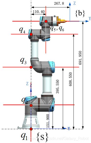
如图所示是UR3机械臂的自由度分布和尺寸。

UR3尺寸示意图：

下面把前面实现的算法应用在六轴UR3机械臂的逆解。我们分为以下几步来做

• 首先是在测量机械臂在初始状态时各个轴线在基座坐标系的表达，
• 其次是建立任务坐标系，工具坐标系等，确定运动轨迹的描述，
• 然后把轨迹的数据输入到逆解算法，计算出各个关节的位置，
• 根据逆解的关节数据进行运动仿真，看末端是否走出了期望的轨迹。

（1）初始状态螺旋轴表示

如下图所示，是UR3机械臂的连杆参数。假设图示构型为机械臂的初始状态，每个轴线上的一点$q_i$如下图所示。

在基座坐标系{s}下各轴的方向向量为和选定的$q_i$为

${\omega }_1=[0,0,1{]}^T,{\omega }_2=[0,1,0{]}^T,{\omega }_3=[0,1,0{]}^T,{\omega }_4=[0,1,0{]}^T,{\omega }_5=[0,0,1{]}^T,{\omega }_6=[0,1,0{]}^T$.

$q_1=[0,0,0{]}^T,q_2=[0,0,151.900],q_3=[0,0,395.550{]}^T,q_4=[213,0,395.55{]}^T,q_5=q_6=[213,110.4,478.95{]}^T$.

这里6个轴都是纯转动轴，根据旋量理论，各个轴的规范化螺旋轴矢量为
$$S_i=[{\omega }_i,-{\omega }_i\times q_i{]}^T$$

（2）轨迹点描述

UR3初始状态示意图：

我们设定机器人的初始状态如上图所示。末端初始构型为
$$M=\left[\begin{array}{cccc}1& 0& 0& 213\\ 0& 1& 0& 267.8\\ 0& 0& 1& 478.95\\ 0& 0& 0& 1\end{array}\right]$$
我们对机器人进行任务规划时，其末端运动轨迹一般不会在机器人基坐标系{s}里表示，通常会在任务坐标系{w}里表示，这两个坐标系的变换为
$$T_{sw}=\left[\begin{array}{cccc}1& 0& 0& -75\\ 0& 0& 0& 300\\ 0& 0& 1& 100\\ 0& 0& 0& 1\end{array}\right]$$

我们要做实验是，让机器人末端从设定的初始状态运动到A(125,75,60), B(85,75,100), C(65,75,100)的位置，并且刀具轴线垂直于这些点所在的平面。这里我们先不考虑速规划和姿态插补，我们只考虑我们逆解的关节位置能否使机械臂末端从初始状态到达指定这3个点，要求是末端刀轴垂直于轨迹点所在平面。期望位姿（构型）用齐次矩阵表示，在任务坐标系下可表示为，
$$\begin{gathered} T_{wA}=\left[\begin{array}{cccc}cos(\pi /2)& -sin(\pi /2)& 0& 125\\ sin(\pi /2)& cos(\pi /2)& 0& 75\\ 0& 0& 1& 60\\ 0& 0& 0& 1\end{array}\right], \\ {T}_{wB}=\left[\begin{array}{cccc}1& 0& 0& 85\\ 0& cos(-\pi /2)& -sin(-\pi /2)& 75\\ 0& sin(-\pi /2)& cos(-\pi /2)& 100\\ 0& 0& 0& 1\end{array}\right] \\ {T}_{wC}=\left[\begin{array}{cccc}1& 0& 0& 65\\ 0& cos(-\pi /2)& -sin(-\pi /2)& 75\\ 0& sin(-\pi /2)& cos(-\pi /2)& 100\\ 0& 0& 0& 1\end{array}\right], \end{gathered}$$

（3）逆解关节位置

我们调用IKinSpaceNR()函数来逆解关节，还需要把上面的参数和坐标转换一下，使得与逆解函数接受的参数含义一致。

用matlab处理一下，

clc
clear
%Slist
w1=[0;0;1];
w2=[0;1;0];
w3=[0;1;0];
w4=[0;1;0];
w5=[0;0;1];
w6=[0;1;0];
q1=[0;0;0];
q2=[0;0;151.900];
q3=[0;0;395.55];
q4=[213;0;395.55];
q5=[213;110.4;478.95];
q6=[213;110.4;478.95];
S1=[w1;cross(-w1,q1)];
S2=[w2;cross(-w2,q2)];
S3=[w3;cross(-w3,q3)];
S4=[w4;cross(-w4,q4)];
S5=[w5;cross(-w5,q5)];
S6=[w6;cross(-w6,q6)];
Slist=[S1,S2,S3,S4,S5,S6];
%初始构型
M=[1,0 , 0 ,213;
    0 ,1 ,0 ,267.8;
    0,0,1,478.95;
    0,0,0,1];
% M=[1,0 , 0 ,327.5853;
%     0 ,1 ,0 ,332.8;
%     0,0,1,364.9;
%     0,0,0,1];
%期望构型
TwA=[cos(pi/2),-sin(pi/2),0,125;
    sin(pi/2),cos(pi/2),0,75;
    0,0,1,60;
    0,0,0,1];
TwB=[1,0,0,85;
    0,cos(-pi/2),-sin(-pi/2),75;
    0,sin(-pi/2),cos(-pi/2),100;
    0,0,0,1];
TwC=[1,0,0,65;
    0,cos(-pi/2),-sin(-pi/2),75;
    0,sin(-pi/2),cos(-pi/2),100;
    0,0,0,1];
 %基坐标系{s}到任务坐标系{w}的变换
  Tsw=[1,0,0,-75;
        0,1,0,300;
        0,0,1,100;
        0,0,0,1];
    TsA= Tsw*TwA;
    TsB=Tsw*TwB;
    TsC=Tsw*TwC;

%参数结果
display(Slist);
display(M);
display(TsA);
display(TsB);
display(TsC);

各参数结果如下

Slist =
         0         0         0         0         0         0
         0    1.0000    1.0000    1.0000         0    1.0000
    1.0000         0         0         0    1.0000         0
         0 -151.9000 -395.5500 -395.5500  110.4000 -478.9500
         0         0         0         0 -213.0000         0
         0         0         0  213.0000         0  213.0000

M =
    1.0000         0         0  213.0000
         0    1.0000         0  267.8000
         0         0    1.0000  478.9500
         0         0         0    1.0000

TsA =
    0.0000   -1.0000         0   50.0000
    1.0000    0.0000         0  375.0000
         0         0    1.0000  160.0000
         0         0         0    1.0000

TsB =
    1.0000         0         0   10.0000
         0    0.0000    1.0000  375.0000
         0   -1.0000    0.0000  200.0000
         0         0         0    1.0000
TsC =
    1.0000         0         0  -10.0000
         0    0.0000    1.0000  375.0000
         0   -1.0000    0.0000  200.0000
         0         0         0    1.0000

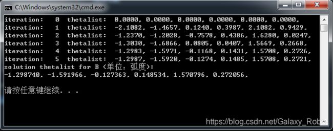
设置误差 姿态误差eomg = 1.0E-4，位置误差 ev = 1.0E-3，调用逆解函数，计算得到ABC这3点对应的3组关节变量如下

A点对应的关节量迭代过程及结果

B点对应的关节量迭代过程及结果

C点对应的关节量迭代过程及结果

（4）运动仿真

使用3D模型进行运动仿真，从初始位置运动到A点

从初始位置运动到B点

从初始位置运动到C点

小结

• 当逆运动学的解析解不存在时使用数值迭代法，求解逆运动学方程的步骤与牛顿-拉普森相似，都需要一组关节变量的初始值。存在多解的时候，迭代的效率很大程度上依赖于初始值，迭代法可以求得最靠近初始值的解。每次迭代的形式如下

$${\theta }^{i+1}={\theta }^i+J^{†}({\theta }^i)\mathcal{V},$$

这里$J^{†}$是雅可比$J(\theta )$的伪逆矩阵，$\mathcal{V}$是运动旋量，表示末端单位时间内从构型$T({\theta }^i)$向构型$T_{sd}$的运动。

• 为了使逆运动学的数值迭代法收敛，初始值与解应该足够靠近。当从机器人初始位置开始是可以满足条件的，该位置的末端构型和关节量都已知，同时要保证末端期望$T_{sd}$缓慢变化，这与逆运动学计算的频率有关。实际应用中从一个位置到另一个位置是进行位置和姿态插补的，这很容易保证每次计算逆运动学末端期望$T_{sd}$缓慢变化。机器人运动过程中，前一时间步（插补周期）计算出的解${\theta }_d$作为下一个时间步计算新的$T_{s}d$的迭代初值。
• 值得注意的是，前面的UR3的例子中，如果直接从下图的构型作为初始状态，A点作为期望位置且刀轴垂直A所在平面，迭代是不收敛的，无法求得正确解，因为，期望位置和初始位置相差太远了，同时这也是一个奇异位置。接下来我们再研究机器人末端的位置和姿态插补，就可以让机器人末端走连续的轨迹了。

---

参考文献

Kenvin M. Lynch , Frank C. Park, Modern Robotics Mechanics,Planning , and Control. May 3, 2017