机器学习10-信用卡反欺诈模型

1.数据准备

# 信用卡反欺诈模型
# 识别数据中的虚假信息
import pandas as pd
import numpy as np
import matplotlib.pyplot as plt

# 数据准备
# 1.加载数据
data = pd.read_csv('data/creditcard.csv',delimiter=',')

print(data.shape)
print(data.head(5))
# 样本类别分布情况
print(data['Class'].value_counts())
# 通过条形图形式，查看数据中两种样本类别的数量情况
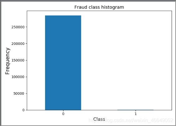
plt.subplots(1,1,figsize = (7,5))
count_classes = pd.value_counts(data['Class'],sort=True).sort_index()
count_classes.plot(kind='bar')
plt.title('Fraud class histogram',fontsize=13)
plt.xlabel('Class',fontsize=13)
plt.ylabel('Frequency',fontsize=15)
# 坐标轴变名
plt.xticks(rotation=0)
plt.show()

# 从图中可以看出，绝大部分样本的类别为“0”，即信用数据可信，仅有极少数的样本类别为“1”，
# 即存在欺诈的情况。 并且数据是极度有偏的

2.数据采样

# 数据采样
# 不平衡数据的训练集与测试的分割方法
data = data.drop(['Time'], axis=1)
# 1.按照被解释变量进行分层超额抽样
# 使用sklearn.model_selection中的StratifiedShuffleSplit做训练集和测试集的划分，该方法先将数据集打乱，
# 之后根据参数设置划分出train/test对，同时可以保证每组划分中类别比例相同。
X = np.array(data.loc[:, :'V28'])
y = np.array(data['Class'])
# n_splits=1表示随机取一次
sess = StratifiedShuffleSplit(n_splits=1, test_size=0.4, random_state=0)

for train_index, test_index in sess.split(X, y):
    print(len(train_index))  # 170884
    # 数据集的分割
    X_train, X_test = X[train_index], X[test_index]
    y_train, y_test = y[train_index], y[test_index]

print('train_size:%s' % len(y_train),
      'test_size:%s' % len(y_test))  # train_size:170884 test_size:113923

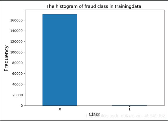
plt.figure(figsize=(7, 5))
count_classes = pd.value_counts(y_train, sort=True)
count_classes.plot(kind='bar')
plt.title("The histogram of fraud class in trainingdata ", fontsize=13)
plt.xlabel("Class", fontsize=13)
plt.ylabel("Frequency", fontsize=15)
plt.xticks(rotation=0)
plt.show()
# 从训练集的两种类别的直方图来看，“0”类数据远多于“1”类数据，数据存在不平衡现象，在建模之前需要进行处理

# 2.过采样平衡样本
# 随机过采样
ros = RandomOverSampler(random_state=0)
# SMOTE过采样
sos = SMOTE(random_state=0)
# 综合过采样
kos = SMOTETomek(random_state=0)

X_ros, y_ros = ros.fit_sample(X_train, y_train)
X_sos, y_sos = sos.fit_sample(X_train, y_train)
X_kos, y_kos = kos.fit_sample(X_train, y_train)

print('ros:%s,sos:%s,kos:%s' % (len(y_ros), len(y_sos), len(y_kos)))

a = pd.DataFrame(y_ros)
print(a[0].value_counts())

284807, 31)
   Time        V1        V2        V3  ...       V27       V28  Amount  Class
0   0.0 -1.359807 -0.072781  2.536347  ...  0.133558 -0.021053  149.62      0
1   0.0  1.191857  0.266151  0.166480  ... -0.008983  0.014724    2.69      0
2   1.0 -1.358354 -1.340163  1.773209  ... -0.055353 -0.059752  378.66      0
3   1.0 -0.966272 -0.185226  1.792993  ...  0.062723  0.061458  123.50      0
4   2.0 -1.158233  0.877737  1.548718  ...  0.219422  0.215153   69.99      0
[5 rows x 31 columns]
0    284315
1       492
Name: Class, dtype: int64
170884
train_size:170884 test_size:113923
ros:341178,sos:341178,kos:341178
1    170589
0    170589
Name: 0, dtype: int64

3.建模与调参

# 建模与调参
# 过采样后，两类样本均衡，下面将对直接划分的训练集和三种过采样方法得到的数据集建立决策树模型进行预测，
# 选择预测效果好的数据集进行后续建模
clf = DecisionTreeClassifier(criterion='gini',random_state=1234)
param_grid = {'max_depth':[3,4,5,6],',max_lesf_nodes':[4,6,8,10,12]}
cv = GridSearchCV(clf,param_grid = param_grid,scoring='f1')

data = [[X_train,y_train],
        [X_ros,y_ros],
        [X_sos,y_sos],
        [X_kos,y_kos]]
# 训练模型
for features,labels in data:
    cv.fit(features,labels)
    pred_test = cv.predict(X_test)

    print('auc:%.3f' % roc_auc_score(y_test, pred_test),
          'recall:%.3f' % recall_score(y_test, pred_test),
          'precision:%.3f' % precision_score(y_test, pred_test))
# 经结果易得，随机过采样的数据集得到的auc值最高

# 利用该数据建立预测模型
train_data = X_ros
train_target = y_ros
test_target = y_test
test_data = X_test

# 逻辑回归
lr = LogisticRegression(C = 1, penalty = 'l1')
lr.fit(train_data,train_target)
test_est = lr.predict(test_data)
print("Logistic Regression accuracy:")
# 分类报告
print(classification_report(test_target,test_est))
fpr_test, tpr_test, th_test = roc_curve(test_target, test_est)
# auc值
print('Logistic Regression AUC: %.4f' %auc(fpr_test, tpr_test))

# 随机森林
rf = RandomForestClassifier(criterion = 'entropy',max_depth = 10,n_estimators = 15,
                            max_features = 0.6,min_samples_split = 50)
rf.fit(train_data, train_target)
test_est = rf.predict(test_data)
print("Random Forest accuracy:")
print(classification_report(test_target,test_est))
fpr_test, tpr_test, th_test = roc_curve(test_target, test_est)
print('Random Forest AUC: %.4f' %auc(fpr_test, tpr_test))

# GBDT
gb = GradientBoostingClassifier(loss = 'exponential',learning_rate = 0.2,n_estimators = 40,
                                       max_depth = 3,min_samples_split = 30)
gb.fit(train_data, train_target)
test_est = gb.predict(test_data)
print("GradientBoosting accuracy:")
print(classification_report(test_target,test_est))
fpr_test, tpr_test, th_test = roc_curve(test_target, test_est)
print('GradientBoosting AUC : %.4f' %auc(fpr_test, tpr_test))

# 寻找最优参数-参数的范围设定对搜索结果起着重要作用，并且在搜索时仅能搭建出局部最优解，而非全局最优解

# 随机森林
param_grid = {
    'criterion':['entropy','gini'],
    'max_depth':[8,10,12],
    'n_estimators':[11,13,15],
    'max_features':[0.3,0.4,0.5],
    'min_samples_split':[4,8,12]
}

rfc = RandomForestClassifier()
rfccv = GridSearchCV(estimator = rfc, param_grid = param_grid, scoring = 'roc_auc', cv = 4)
rfccv.fit(train_data, train_target)
test_est = rfccv.predict(test_data)
print("Random Forest accuracy:")
# 分类报告
print(classification_report(test_target,test_est))
fpr_test, tpr_test, th_test = roc_curve(test_target, test_est)
print('Random Forest AUC: %.4f' %auc(fpr_test, tpr_test))

print('最优参数模型为:\n',rfccv.best_params_)


# GBDT
param_grid = {
    'learning_rate':[0.1,0.3,0.5],
    'n_estimators':[15,20,30],
    'max_depth':[1,2,3],
    'min_samples_split':[12,16,20]
}

gbc = GradientBoostingClassifier()
gbccv = GridSearchCV(estimator = gbc, param_grid = param_grid, scoring = 'roc_auc', cv = 4)
gbccv.fit(train_data, train_target)
test_est = gbccv.predict(test_data)
print("Gradient Boosting accuracy:")
# 分类报告
print(classification_report(test_target,test_est))
fpr_test, tpr_test, th_test = roc_curve(test_target, test_est)
print('Gradient Boosting AUC : %.4f' %auc(fpr_test, tpr_test))

print('最优参数模型:\n',gbccv.best_params_)

最终代码

import matplotlib.pyplot as plt
import numpy as np
# 信用卡反欺诈模型
# 识别数据中的虚假信息
import pandas as pd
from imblearn.combine import SMOTETomek
# 过采样
from imblearn.over_sampling import RandomOverSampler, SMOTE
from sklearn.ensemble import RandomForestClassifier, GradientBoostingClassifier
from sklearn.linear_model import LogisticRegression
from sklearn.metrics import (auc, roc_auc_score, precision_score, roc_curve, recall_score, classification_report)
from sklearn.model_selection import GridSearchCV
from sklearn.model_selection import StratifiedShuffleSplit
from sklearn.tree import DecisionTreeClassifier

# 数据准备
# 1.加载数据
data = pd.read_csv('data/creditcard.csv', delimiter=',')

print(data.shape)
print(data.head(5))
# 样本类别分布情况
print(data['Class'].value_counts())
# 通过条形图形式，查看数据中两种样本类别的数量情况
plt.subplots(1, 1, figsize=(7, 5))
count_classes = pd.value_counts(data['Class'], sort=True).sort_index()
count_classes.plot(kind='bar')
plt.title('Fraud class histogram', fontsize=13)
plt.xlabel('Class', fontsize=13)
plt.ylabel('Frequency', fontsize=15)
# 坐标轴变名
plt.xticks(rotation=0)
plt.show()

# 从图中可以看出，绝大部分样本的类别为“0”，即信用数据可信，仅有极少数的样本类别为“1”，
# 即存在欺诈的情况。 并且数据是极度有偏的

# 数据采样
# 不平衡数据的训练集与测试的分割方法
data = data.drop(['Time'], axis=1)
# 1.按照被解释变量进行分层超额抽样
# 使用sklearn.model_selection中的StratifiedShuffleSplit做训练集和测试集的划分，该方法先将数据集打乱，
# 之后根据参数设置划分出train/test对，同时可以保证每组划分中类别比例相同。
X = np.array(data.loc[:, :'V28'])
y = np.array(data['Class'])
# n_splits=1表示随机取一次
sess = StratifiedShuffleSplit(n_splits=1, test_size=0.4, random_state=0)

for train_index, test_index in sess.split(X, y):
    print(len(train_index))  # 170884
    # 数据集的分割
    X_train, X_test = X[train_index], X[test_index]
    y_train, y_test = y[train_index], y[test_index]

print('train_size:%s' % len(y_train),
      'test_size:%s' % len(y_test))  # train_size:170884 test_size:113923

plt.figure(figsize=(7, 5))
count_classes = pd.value_counts(y_train, sort=True)
count_classes.plot(kind='bar')
plt.title("The histogram of fraud class in trainingdata ", fontsize=13)
plt.xlabel("Class", fontsize=13)
plt.ylabel("Frequency", fontsize=15)
plt.xticks(rotation=0)
plt.show()
# 从训练集的两种类别的直方图来看，“0”类数据远多于“1”类数据，数据存在不平衡现象，在建模之前需要进行处理

# 2.过采样平衡样本
# 随机过采样
ros = RandomOverSampler(random_state=0)
# SMOTE过采样
sos = SMOTE(random_state=0)
# 综合过采样
kos = SMOTETomek(random_state=0)

X_ros, y_ros = ros.fit_sample(X_train, y_train)
X_sos, y_sos = sos.fit_sample(X_train, y_train)
X_kos, y_kos = kos.fit_sample(X_train, y_train)

print('ros:%s,sos:%s,kos:%s' % (len(y_ros), len(y_sos), len(y_kos)))

a = pd.DataFrame(y_ros)
print(a[0].value_counts())

# 建模与调参
# 过采样后，两类样本均衡，下面将对直接划分的训练集和三种过采样方法得到的数据集建立决策树模型进行预测，
# 选择预测效果好的数据集进行后续建模
clf = DecisionTreeClassifier(criterion='gini', random_state=1234)
param_grid = {'max_depth': [3, 4, 5, 6], ',max_lesf_nodes': [4, 6, 8, 10, 12]}
cv = GridSearchCV(clf, param_grid=param_grid, scoring='f1')

data = [[X_train, y_train],
        [X_ros, y_ros],
        [X_sos, y_sos],
        [X_kos, y_kos]]
# 训练模型
for features, labels in data:
    cv.fit(features, labels)
    pred_test = cv.predict(X_test)
    print('auc:%.3f' % roc_auc_score(y_test, pred_test),
          'recall:%.3f' % recall_score(y_test, pred_test),
          'precision:%.3f' % precision_score(y_test, pred_test))
# 经结果易得，随机过采样的数据集得到的auc值最高

# 利用该数据建立预测模型
train_data = X_ros
train_target = y_ros
test_target = y_test
test_data = X_test

# 逻辑回归
lr = LogisticRegression(C=1, penalty='l1')
lr.fit(train_data, train_target)
test_est = lr.predict(test_data)
print("Logistic Regression accuracy:")
# 分类报告
print(classification_report(test_target, test_est))
fpr_test, tpr_test, th_test = roc_curve(test_target, test_est)
# auc值
print('Logistic Regression AUC: %.4f' % auc(fpr_test, tpr_test))

# 随机森林
rf = RandomForestClassifier(criterion='entropy', max_depth=10, n_estimators=15,
                            max_features=0.6, min_samples_split=50)
rf.fit(train_data, train_target)
test_est = rf.predict(test_data)
print("Random Forest accuracy:")
print(classification_report(test_target, test_est))
fpr_test, tpr_test, th_test = roc_curve(test_target, test_est)
print('Random Forest AUC: %.4f' % auc(fpr_test, tpr_test))

# GBDT
gb = GradientBoostingClassifier(loss='exponential', learning_rate=0.2, n_estimators=40,
                                max_depth=3, min_samples_split=30)
gb.fit(train_data, train_target)
test_est = gb.predict(test_data)
print("GradientBoosting accuracy:")
print(classification_report(test_target, test_est))
fpr_test, tpr_test, th_test = roc_curve(test_target, test_est)
print('GradientBoosting AUC : %.4f' % auc(fpr_test, tpr_test))

# 寻找最优参数-参数的范围设定对搜索结果起着重要作用，并且在搜索时仅能搭建出局部最优解，而非全局最优解

# 随机森林
param_grid = {
    'criterion': ['entropy', 'gini'],
    'max_depth': [8, 10, 12],
    'n_estimators': [11, 13, 15],
    'max_features': [0.3, 0.4, 0.5],
    'min_samples_split': [4, 8, 12]
}

rfc = RandomForestClassifier()
rfccv = GridSearchCV(estimator=rfc, param_grid=param_grid, scoring='roc_auc', cv=4)
rfccv.fit(train_data, train_target)
test_est = rfccv.predict(test_data)
print("Random Forest accuracy:")
# 分类报告
print(classification_report(test_target, test_est))
fpr_test, tpr_test, th_test = roc_curve(test_target, test_est)
print('Random Forest AUC: %.4f' % auc(fpr_test, tpr_test))

print('最优参数模型为:\n', rfccv.best_params_)

# GBDT
param_grid = {
    'learning_rate': [0.1, 0.3, 0.5],
    'n_estimators': [15, 20, 30],
    'max_depth': [1, 2, 3],
    'min_samples_split': [12, 16, 20]
}

gbc = GradientBoostingClassifier()
gbccv = GridSearchCV(estimator=gbc, param_grid=param_grid, scoring='roc_auc', cv=4)
gbccv.fit(train_data, train_target)
test_est = gbccv.predict(test_data)
print("Gradient Boosting accuracy:")
# 分类报告
print(classification_report(test_target, test_est))
fpr_test, tpr_test, th_test = roc_curve(test_target, test_est)
print('Gradient Boosting AUC : %.4f' % auc(fpr_test, tpr_test))

print('最优参数模型:\n', gbccv.best_params_)