机器学习 | 网络搜索及可视化

相关文章：

机器学习 | 目录

监督学习 | 决策树之网络搜索

监督学习 | SVM 之线性支持向量机原理

监督学习 | SVM 之非线性支持向量机原理

监督学习 | SVM 之支持向量机Sklearn实现

1. 网络搜索

网络搜索（Grid Search）：一种调参方法，利用穷举搜索，在所有候选的参数选择中，通过循环便利，尝试每一种可能性，表现最好的参数就是最终的结果。其原理就是在数组里找最大值。（为什么叫网格搜索？以有两个参数的模型为例，参数 a 有 3 种可能，参数 b 有 4 种可能，把所有可能性列出来，可以表示成一个$3\times 4$的表格，其中每个cell就是一个网格，循环过程就像是在每个网格里遍历、搜索，所以叫grid search）^[1]

1.1 简单网络搜索

考虑一个具有 RBF（径向基函数）核的核 SVM 的例子。

我们可以使用 Python 实现一个简单的网络搜索，在 2 个参数上使用 for 循环，对每种参数组合分别训练并评估一个分类器：

# naive grid search implementation
from sklearn.datasets import load_iris
from sklearn.model_selection import train_test_split
from sklearn.svm import SVC

iris = load_iris()
X_train, X_test, y_train, y_test = train_test_split(iris.data, iris.target,
                                                    random_state=0)
print("Size of training set: {}   size of test set: {}".format(
      X_train.shape[0], X_test.shape[0]))

best_score = 0

for gamma in [0.001, 0.01, 0.1, 1, 10, 100]:
    for C in [0.001, 0.01, 0.1, 1, 10, 100]:
        # for each combination of parameters, train an SVC
        svm = SVC(gamma=gamma, C=C)
        svm.fit(X_train, y_train)
        # evaluate the SVC on the test set
        score = svm.score(X_test, y_test)
        # if we got a better score, store the score and parameters
        if score > best_score:
            best_score = score
            best_parameters = {'C': C, 'gamma': gamma}

print("Best score: {:.2f}".format(best_score))
print("Best parameters: {}".format(best_parameters))

Size of training set: 112   size of test set: 38
Best score: 0.97
Best parameters: {'C': 100, 'gamma': 0.001}

1.2 参数过拟合的风险与验证集

看到这个结果，是否意味着我们找到了一个在数据集上精度达到 97% 的模型呢？答案是否定的，原因如下：

我们尝试了许多不同的参数，并选择了在测试集上精度最高的那个，但这个精度不一定能推广到新数据上。由于我们使用测试数据继续调参，所以不能再用它来评估模型的好坏。也就是说调参过程的模型得分不能作为最终得分。我们最开始需要将数据划分为训练集和测试集也是因为这个原因。我们需要一个独立的数据集来进行评估，一个在创建模型时没有用到的数据集。

为了解决这个问题，一个方法时再次划分数据，这样我们得到 3 个数据集：用于构建模型的训练集（Training Set），用于选择模型参数的验证集（Validation Set），用于评估所选参数性能的测试集（Testing Set）。如下图所示：

利用验证集选定最佳参数之后，我们可以利用找到的参数设置重新构建一个模型，但是要同时在训练数据和验证数据上进行训练，这样我们可以利用尽可能多的数据来构建模型。其实现如下所示：

from sklearn.svm import SVC
# split data into train+validation set and test set
X_trainval, X_test, y_trainval, y_test = train_test_split(
    iris.data, iris.target, random_state=0)
# split train+validation set into training and validation sets
X_train, X_valid, y_train, y_valid = train_test_split(
    X_trainval, y_trainval, random_state=1)
print("Size of training set: {}   size of validation set: {}   size of test set:"
      " {}\n".format(X_train.shape[0], X_valid.shape[0], X_test.shape[0]))

best_score = 0

for gamma in [0.001, 0.01, 0.1, 1, 10, 100]:
    for C in [0.001, 0.01, 0.1, 1, 10, 100]:
        # for each combination of parameters train an SVC
        svm = SVC(gamma=gamma, C=C)
        svm.fit(X_train, y_train)
        # evaluate the SVC on the validation set
        score = svm.score(X_valid, y_valid)
        # if we got a better score, store the score and parameters
        if score > best_score:
            best_score = score
            best_parameters = {'C': C, 'gamma': gamma}

# rebuild a model on the combined training and validation set,
# and evaluate it on the test set
svm = SVC(**best_parameters)
svm.fit(X_trainval, y_trainval)
test_score = svm.score(X_test, y_test)
print("Best score on validation set: {:.2f}".format(best_score))
print("Best parameters: ", best_parameters)
print("Test set score with best parameters: {:.2f}".format(test_score))

Size of training set: 84   size of validation set: 28   size of test set: 38

Best score on validation set: 0.96
Best parameters:  {'C': 10, 'gamma': 0.001}
Test set score with best parameters: 0.92

验证集上的最高分数时 96%，这比之前略低，可能是因为我们使用了更少的数据来训练模型（现在 X_train 更小，因为我们对数据集进行了两次划分）。但测试集上的分数（这个分数实际反映了模型的泛化能力）更低，为 92%。因此，我们只能声称对 92% 的新数据正确分类，而不是我们之前认为的 97%！

1.3 带交叉验证的网络搜索

虽然将数据划分为训练集、验证集和测试集的方法（如上所述）是可行的，也相对可用，但这种方法对数据的划分相当敏感。为了得到对泛化性能的更好估计，我们可以使用交叉验证（机器学习 | 模型选择）来评估每种参数组合的性能，而不是仅将数据单次划分为训练集与验证集。整个过程如下所示：

1.3.1 Python 实现

from sklearn.model_selection import cross_val_score

for gamma in [0.001, 0.01, 0.1, 1, 10, 100]:
    for C in [0.001, 0.01, 0.1, 1, 10, 100]:
        # 对每种参数组合都训练一个 SVC
        svm = SVC(gamma=gamma, C=C)
        # 执行交叉验证
        scores = cross_val_score(svm, X_trainval, y_trainval, cv=5)
        # 计算交叉验证平均精度
        score = np.mean(scores)
        # 如果得到更高的分数，则保存该分数和对应的参数
        if score > best_score:
            best_score = score
            best_parameters = {'C': C, 'gamma': gamma}
# 利用训练集和验证集得到最优参数重新构建一个模型
svm = SVC(**best_parameters)
svm.fit(X_trainval, y_trainval)

SVC(C=100, cache_size=200, class_weight=None, coef0=0.0,
    decision_function_shape='ovr', degree=3, gamma=0.01, kernel='rbf',
    max_iter=-1, probability=False, random_state=None, shrinking=True,
    tol=0.001, verbose=False)

选择最优参数的过程如下所示：

交叉验证是在特定数据集上对给定算法进行评估的一种方法，但它通常与网络搜算等参数搜索方法结合使用。因此，许多人使用交叉验证（Cross-validation）这一术语来通俗地指代交叉验证的网络搜素。

1.3.2 Sklearn 实现

由于带交叉验证的网络搜索是一种常用的调参方法，因此 sickit-learn 提供了 GridSearchCV `类，它以评估其（estimator）的形式实现了这种方法。要使用 GridSerachCV 类，首先需要用一个字典指定要搜索的参数，然后 GridSearchCV 会执行所有必要的模型拟合。

sklearn.model_selection.GridSearchCV：（Sklearn 官方文档）

创建网络搜索器：GridSearchCV(estimator, param_grid, cv, return_train_score=False)

其中 estimator 为想要训练的模型，param_grid 为想要训练的参数字典，cv 为交叉验证的折数。

GridSearchCV 包含的方法：

1. fit、predict、score：分别进行拟合、预测和得出泛化性能分数

2. best_params 、 best_score_、best_estimator_：查看最佳参数、所对应的交叉验证平均分数和其对于的最佳模型

3. cv_results_：返回包含网络搜索的结果的字典

字典的键是我们想要尝试的参数设置。如 C 个 gamma 想要尝试的取值为 0.001、 0.01、 0.1、 1 、10 和 100，可以将其转化为下面的字典：

param_grid = {'C': [0.001, 0.01, 0.1, 1, 10, 100],
              'gamma': [0.001, 0.01, 0.1, 1, 10, 100]}
print("Parameter grid:\n{}".format(param_grid))

Parameter grid:
{'C': [0.001, 0.01, 0.1, 1, 10, 100], 'gamma': [0.001, 0.01, 0.1, 1, 10, 100]}

我们现在可以使用模型（SVC）、要搜索的参数网络（param_grid）与要使用的交叉验证策略（比如 5 折分层交叉验证）将 GridSearchCV 类实例化：

from sklearn.model_selection import GridSearchCV
from sklearn.svm import SVC
grid_search = GridSearchCV(SVC(), param_grid, cv=5, return_train_score=True)

GridSearchCV 将使用交叉验证来代替之前用过的划分训练集和验证集方法。但是，我们仍需要将数据划分为训练集和测试集，以避免参数过拟合：

X_train, X_test, y_train, y_test = train_test_split(iris.data, iris.target, random_state=0)

我们创建的 grid_search 对象的行为就像是一个分类器，我们可以对它叫用标准的 fit、predict 和 score 方法。但我们在调用 fit 时，它会对 param_grid 指定的美中参数组合都运行交叉验证：

grid_search.fit(X_train, y_train)

GridSearchCV(cv=5, error_score='raise-deprecating',
             estimator=SVC(C=1.0, cache_size=200, class_weight=None, coef0=0.0,
                           decision_function_shape='ovr', degree=3,
                           gamma='auto_deprecated', kernel='rbf', max_iter=-1,
                           probability=False, random_state=None, shrinking=True,
                           tol=0.001, verbose=False),
             iid='warn', n_jobs=None,
             param_grid={'C': [0.001, 0.01, 0.1, 1, 10, 100],
                         'gamma': [0.001, 0.01, 0.1, 1, 10, 100]},
             pre_dispatch='2*n_jobs', refit=True, return_train_score=True,
             scoring=None, verbose=0)

拟合 GridSearchCV 对象不仅会搜索最佳参数，还会利用得到最佳交叉验证性能的参数在整个训练数据集上自动拟合一个新模型。因此，fit 完成的工作相当于 1.3.1 的代码结果。

GridSerachCV 类提供了一个非常方便的接口，可以用 predic 和 score 方法来访问重新训练过的模型。为了评估找到的最佳参数的泛化能力，我们可以在测试集上调用 score：

print("Test set score: {:.2f}".format(grid_search.score(X_test, y_test)))

Test set score: 0.97

从结果中看出，我们利用交叉验证选择的参数，找到了一个在测试集上精度为 97% 的模型。重要的是，我们没有使用测试集来选择参数。我们找到的参数保存在 best_params属性中，而交叉验证最佳精度（对于这种参数设置，不同划分的平均精度）保存在best_score_中:

print("Best parameters: {}".format(grid_search.best_params_))
print("Best cross-validation score: {:.2f}".format(grid_search.best_score_))

Best parameters: {'C': 100, 'gamma': 0.01}
Best cross-validation score: 0.97

同样，注意不要将 best_score_ 与模型在测试集上调用 score 方法计算得到的泛化性能弄混。使用 score 方法（或者对 predict 方法的输出进行评估）采用的是在整个训练集上训练的模型。而best_score_属性保存的是交叉验证的平均精度，是在训练集上进行交叉验证得到的。

能够访问实际找到的模型，这有时是很有帮助的，比如查看系数或特征重要性。可以使用 best_estimator_ 属性来访问最佳属性对于的模型，它是在整个训练集上训练得到的：

print("Best estimator:\n{}".format(grid_search.best_estimator_))

Best estimator:
SVC(C=100, cache_size=200, class_weight=None, coef0=0.0,
    decision_function_shape='ovr', degree=3, gamma=0.01, kernel='rbf',
    max_iter=-1, probability=False, random_state=None, shrinking=True,
    tol=0.001, verbose=False)

1.4 网络搜索可视化

1.4.1 在网络空间中的搜索

将交叉验证的结果可视化通常有助于理解模型泛化能力对所搜索参数的依赖关系。由于运行网络搜索的计算成本相当高，所以通常最好从比较稀疏且较小的网络开始搜索。然后我们可以检查交叉验证网络搜索的结果，可能也会扩展搜索范围。

网络搜索的结果可以在 cv_results_ 属性中找到，它是一个字典，其中保存了搜索的所有内容。

可以将其转换为 DataFrame 后再查看：

import pandas as pd
# convert to Dataframe
results = pd.DataFrame(grid_search.cv_results_)
# show the first 5 rows
display(results.head())

	mean_fit_time	std_fit_time	mean_score_time	std_score_time	param_C	param_gamma	params	split0_test_score	split1_test_score	split2_test_score	...	mean_test_score	std_test_score	rank_test_score	split0_train_score	split1_train_score	split2_train_score	split3_train_score	split4_train_score	mean_train_score	std_train_score
0	0.001317	0.000458	0.001943	0.001243	0.001	0.001	{'C': 0.001, 'gamma': 0.001}	0.375	0.347826	0.363636	...	0.366071	0.011371	22	0.363636	0.370787	0.366667	0.366667	0.362637	0.366079	0.002852
1	0.001284	0.000543	0.001329	0.001086	0.001	0.01	{'C': 0.001, 'gamma': 0.01}	0.375	0.347826	0.363636	...	0.366071	0.011371	22	0.363636	0.370787	0.366667	0.366667	0.362637	0.366079	0.002852
2	0.000582	0.000024	0.000272	0.000020	0.001	0.1	{'C': 0.001, 'gamma': 0.1}	0.375	0.347826	0.363636	...	0.366071	0.011371	22	0.363636	0.370787	0.366667	0.366667	0.362637	0.366079	0.002852
3	0.000606	0.000021	0.000279	0.000012	0.001	1	{'C': 0.001, 'gamma': 1}	0.375	0.347826	0.363636	...	0.366071	0.011371	22	0.363636	0.370787	0.366667	0.366667	0.362637	0.366079	0.002852
4	0.000661	0.000032	0.000294	0.000033	0.001	10	{'C': 0.001, 'gamma': 10}	0.375	0.347826	0.363636	...	0.366071	0.011371	22	0.363636	0.370787	0.366667	0.366667	0.362637	0.366079	0.002852

5 rows × 22 columns

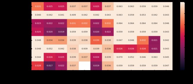
results 中的每一行对应一种特定的参数设置（results[‘params’]）。对于每种参数设置，交叉验证所有划分的结果都被记录下来，所有划分的平均值和标准差也被记录下来。由于我们搜索的是一个二维参数网络（C 和 gamma），所以最适合用热力可视化。我们首先提取平均验证分数，然后改变分数数组的形状，使其坐标轴分别对应于 C 和 gamma：

import mglearn

scores = np.array(results.mean_test_score).reshape(6, 6)

# plot the mean cross-validation scores
mglearn.tools.heatmap(scores, xlabel='gamma', xticklabels=param_grid['gamma'],
                      ylabel='C', yticklabels=param_grid['C'], cmap="viridis")

热图中每个点对于运行一次交叉验证以及一种特定的参数设置。颜色表示交叉验证的精度：浅色表示高精度，深色表示低精度。

可以看到，SVC 对参数设置非常敏感。对于许多参数这只，精度都在 40% 左右，这是非常糟糕的；对于其他参数设置，精度约为 96%。

我们可以从这张图中看出一下两点：

首先，我们调整的参数对于获得良好的性能非常重要。这两个参数（C 和 gamma）都很重要，约为调节它们可以将精度从 40% 提高到 96%。

此外，在我们选择的参数范围中也可以看到输出发生了明显的变化。同样重要的是要注意，参数的范围要足够大：每个参数的最佳取值不能位于图像的边界上。

1.4.1.1 错误的参数设置和可视化

下面我们来看几张图，其结果不那么理想，因为选择的搜索范围不合适：

import matplotlib.pyplot as plt

fig, axes = plt.subplots(1, 3, figsize=(13, 5))

param_grid_linear = {'C': np.linspace(1, 2, 6),
                     'gamma':  np.linspace(1, 2, 6)}

param_grid_one_log = {'C': np.linspace(1, 2, 6),
                      'gamma':  np.logspace(-3, 2, 6)}

param_grid_range = {'C': np.logspace(-3, 2, 6),
                    'gamma':  np.logspace(-7, -2, 6)}

for param_grid, ax in zip([param_grid_linear, param_grid_one_log,
                           param_grid_range], axes):
    grid_search = GridSearchCV(SVC(), param_grid, cv=5)
    grid_search.fit(X_train, y_train)
    scores = grid_search.cv_results_['mean_test_score'].reshape(6, 6)

    # plot the mean cross-validation scores
    scores_image = mglearn.tools.heatmap(
        scores, xlabel='gamma', ylabel='C', xticklabels=param_grid['gamma'],
        yticklabels=param_grid['C'], cmap="viridis", ax=ax)

plt.colorbar(scores_image, ax=axes.tolist())

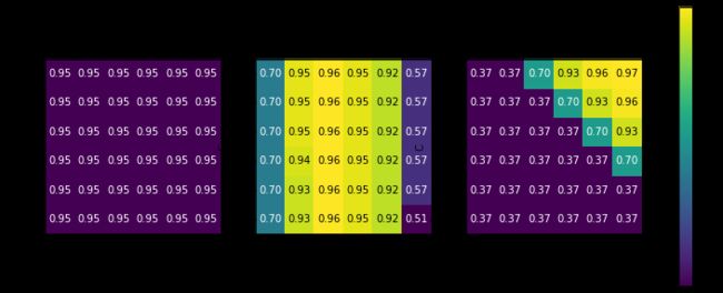
第一张图没有任何变化，整个参数网络的颜色相同。这种情况，是由参数 C 和 gamma 不正确的缩放以及不正确的范围造成的。但如果对于不同的参数设置都看不到精度的变化，也可能是因为这个参数根本不重要。通常最好在开始时尝试非常极端的值，以观察参数是否会导致精度发生变化。

第二张图显示的是垂直条形模式。这表示只有 gamma 的设置对精度有影响。这可能意味着 gamma 参数的搜索范围是我们所关心的，而 C 参数并不是——也可能意味着 C 参数并不重要。

第三章图中 C 和 gamma 对于的精度都有变化。但可以看到，在图像的整个左下角都没有发生什么有趣的事情。我们在后面的网络搜索中可以不考虑非常小的值。最佳参数设置出现在右上角。由于最佳参数位于图像的边界，所以我们可以认为，在这个边界之外可能还有更好的取值，我们可能希望改变搜索范围以包含这一区域内的更多参数。

基于交叉验证分数来调节参数网络是非常好的，也是探索不同参数等莪重要性的好方法。但是，不应该在最终测试集上测试不同的参数范围——前面说过，只有确切知道了想要使用的模型，才能对测试集进行评估。

1.4.2 在非网络空间的搜索

在某些情况下，尝试所有参数的所有可能组合（正如 GridSearchCV 所做的那样）并不是一个好主意。

例如，SVC 有一个 kernel 参数，根据所选择的 kernel（内核），其他桉树也是与之相关的。如果 kernal=‘linear’，那么模型是线性的，只会用到 C 参数。如果 kernal=‘rbf’，则需要使用 C 和 gamma 两个参数（但用不到类似 degree 的其他参数）。在这种情况下，搜索 C、gamma 和 kernel 所有可能的组合没有意义：如果 kernal=‘linear’，那么 gamma 是用不到的，尝试 gamma 的不同取值将会浪费时间。为了处理这种“条件”（conditional）参数，GridSearchCV 的 param_grid 可以是字典组成的列表（a list of dictionaries）。列表中的每个字典可以扩展为一个独立的网络。包含内核与参数的网络搜索可能如下所示：

param_grid = [{'kernel': ['rbf'],
               'C': [0.001, 0.01, 0.1, 1, 10, 100],
               'gamma': [0.001, 0.01, 0.1, 1, 10, 100]},
              {'kernel': ['linear'],
               'C': [0.001, 0.01, 0.1, 1, 10, 100]}]
print("List of grids:\n{}".format(param_grid))

List of grids:
[{'kernel': ['rbf'], 'C': [0.001, 0.01, 0.1, 1, 10, 100], 'gamma': [0.001, 0.01, 0.1, 1, 10, 100]}, {'kernel': ['linear'], 'C': [0.001, 0.01, 0.1, 1, 10, 100]}]

在第一个网络里，kernel 参数始终等于’rbf’（注意 kernel 是一个长度为1 的列表），而 C 和 gamma 都是变化的。在第二个网络里，kernel 参数始终等于’linear’，只有 C 是变化的。下面为来应用这个更加复杂的参数搜索：

grid_search = GridSearchCV(SVC(), param_grid, cv=5, return_train_score=True)
grid_search.fit(X_train, y_train)
print("Best parameters: {}".format(grid_search.best_params_))
print("Best cross-validation score: {:.2f}".format(grid_search.best_score_))

Best parameters: {'C': 100, 'gamma': 0.01, 'kernel': 'rbf'}
Best cross-validation score: 0.97


//anaconda3/lib/python3.7/site-packages/sklearn/model_selection/_search.py:813: DeprecationWarning: The default of the `iid` parameter will change from True to False in version 0.22 and will be removed in 0.24. This will change numeric results when test-set sizes are unequal.
  DeprecationWarning)

我们再次查看 cv_results_。正如所料，如果 kernel 等于’linear’，那么只有 C 是变化的：

results = pd.DataFrame(grid_search.cv_results_)
display(results.T)

	0	1	2	3	4	5	6	7	8	9	...	32	33	34	35	36	37	38	39	40	41
mean_fit_time	0.00216327	0.000975418	0.000895834	0.000586128	0.00068078	0.000671005	0.000685596	0.000640059	0.000607777	0.000593805	...	0.000373602	0.000664568	0.00153198	0.000837708	0.000766277	0.000468493	0.000435066	0.000450134	0.000438309	0.000494576
std_fit_time	0.00140655	0.000492319	0.000402465	7.89536e-06	9.49278e-05	6.87857e-05	0.000189589	2.10245e-05	4.78872e-05	3.52042e-05	...	1.16059e-05	0.000257769	0.000392493	1.99011e-05	0.000322841	6.2482e-06	5.08608e-05	6.50786e-05	5.02317e-05	9.95536e-05
mean_score_time	0.00120344	0.00066967	0.000573587	0.000267696	0.000307798	0.000287628	0.000324154	0.000369263	0.00028758	0.000271845	...	0.000237846	0.000820303	0.000544834	0.000293589	0.000356293	0.000244951	0.000246334	0.00025301	0.000280857	0.000261641
std_score_time	0.000699682	0.000710382	0.000403534	6.3643e-06	6.30153e-05	2.14702e-05	6.90788e-05	0.000185553	3.8449e-05	1.27472e-05	...	1.7688e-06	0.00111757	0.000110992	4.59797e-05	0.000161759	1.7688e-06	8.52646e-06	3.69834e-05	8.52978e-05	2.57724e-05
param_C	0.001	0.001	0.001	0.001	0.001	0.001	0.01	0.01	0.01	0.01	...	100	100	100	100	0.001	0.01	0.1	1	10	100
param_gamma	0.001	0.01	0.1	1	10	100	0.001	0.01	0.1	1	...	0.1	1	10	100	NaN	NaN	NaN	NaN	NaN	NaN
param_kernel	rbf	rbf	rbf	rbf	rbf	rbf	rbf	rbf	rbf	rbf	...	rbf	rbf	rbf	rbf	linear	linear	linear	linear	linear	linear
params	{'C': 0.001, 'gamma': 0.001, 'kernel': 'rbf'}	{'C': 0.001, 'gamma': 0.01, 'kernel': 'rbf'}	{'C': 0.001, 'gamma': 0.1, 'kernel': 'rbf'}	{'C': 0.001, 'gamma': 1, 'kernel': 'rbf'}	{'C': 0.001, 'gamma': 10, 'kernel': 'rbf'}	{'C': 0.001, 'gamma': 100, 'kernel': 'rbf'}	{'C': 0.01, 'gamma': 0.001, 'kernel': 'rbf'}	{'C': 0.01, 'gamma': 0.01, 'kernel': 'rbf'}	{'C': 0.01, 'gamma': 0.1, 'kernel': 'rbf'}	{'C': 0.01, 'gamma': 1, 'kernel': 'rbf'}	...	{'C': 100, 'gamma': 0.1, 'kernel': 'rbf'}	{'C': 100, 'gamma': 1, 'kernel': 'rbf'}	{'C': 100, 'gamma': 10, 'kernel': 'rbf'}	{'C': 100, 'gamma': 100, 'kernel': 'rbf'}	{'C': 0.001, 'kernel': 'linear'}	{'C': 0.01, 'kernel': 'linear'}	{'C': 0.1, 'kernel': 'linear'}	{'C': 1, 'kernel': 'linear'}	{'C': 10, 'kernel': 'linear'}	{'C': 100, 'kernel': 'linear'}
split0_test_score	0.375	0.375	0.375	0.375	0.375	0.375	0.375	0.375	0.375	0.375	...	0.958333	0.916667	0.875	0.541667	0.375	0.916667	0.958333	1	0.958333	0.958333
split1_test_score	0.347826	0.347826	0.347826	0.347826	0.347826	0.347826	0.347826	0.347826	0.347826	0.347826	...	1	1	0.956522	0.521739	0.347826	0.826087	0.913043	0.956522	1	1
split2_test_score	0.363636	0.363636	0.363636	0.363636	0.363636	0.363636	0.363636	0.363636	0.363636	0.363636	...	1	1	1	0.590909	0.363636	0.818182	1	1	1	1
split3_test_score	0.363636	0.363636	0.363636	0.363636	0.363636	0.363636	0.363636	0.363636	0.363636	0.363636	...	0.863636	0.863636	0.818182	0.590909	0.363636	0.772727	0.909091	0.954545	0.909091	0.909091
split4_test_score	0.380952	0.380952	0.380952	0.380952	0.380952	0.380952	0.380952	0.380952	0.380952	0.380952	...	0.952381	0.952381	0.952381	0.619048	0.380952	0.904762	0.952381	0.952381	0.952381	0.952381
mean_test_score	0.366071	0.366071	0.366071	0.366071	0.366071	0.366071	0.366071	0.366071	0.366071	0.366071	...	0.955357	0.946429	0.919643	0.571429	0.366071	0.848214	0.946429	0.973214	0.964286	0.964286
std_test_score	0.0113708	0.0113708	0.0113708	0.0113708	0.0113708	0.0113708	0.0113708	0.0113708	0.0113708	0.0113708	...	0.0495662	0.0519227	0.0647906	0.0356525	0.0113708	0.0547783	0.0332185	0.0223995	0.0338387	0.0338387
rank_test_score	27	27	27	27	27	27	27	27	27	27	...	9	11	17	24	27	21	11	1	3	3
split0_train_score	0.363636	0.363636	0.363636	0.363636	0.363636	0.363636	0.363636	0.363636	0.363636	0.363636	...	0.988636	1	1	1	0.363636	0.886364	0.965909	0.988636	0.988636	0.988636
split1_train_score	0.370787	0.370787	0.370787	0.370787	0.370787	0.370787	0.370787	0.370787	0.370787	0.370787	...	0.977528	1	1	1	0.370787	0.88764	0.977528	0.977528	0.988764	0.988764
split2_train_score	0.366667	0.366667	0.366667	0.366667	0.366667	0.366667	0.366667	0.366667	0.366667	0.366667	...	0.977778	1	1	1	0.366667	0.866667	0.944444	0.977778	0.977778	0.988889
split3_train_score	0.366667	0.366667	0.366667	0.366667	0.366667	0.366667	0.366667	0.366667	0.366667	0.366667	...	1	1	1	1	0.366667	0.755556	0.977778	0.988889	0.988889	1
split4_train_score	0.362637	0.362637	0.362637	0.362637	0.362637	0.362637	0.362637	0.362637	0.362637	0.362637	...	1	1	1	1	0.362637	0.879121	0.967033	0.989011	1	1
mean_train_score	0.366079	0.366079	0.366079	0.366079	0.366079	0.366079	0.366079	0.366079	0.366079	0.366079	...	0.988788	1	1	1	0.366079	0.855069	0.966538	0.984368	0.988813	0.993258
std_train_score	0.00285176	0.00285176	0.00285176	0.00285176	0.00285176	0.00285176	0.00285176	0.00285176	0.00285176	0.00285176	...	0.00999451	0	0	0	0.00285176	0.0503114	0.0121316	0.00548507	0.00702801	0.00550551

23 rows × 42 columns

参考资料

[1] April15 .调参必备—GridSearch网格搜索[EB/OL].https://www.cnblogs.com/ysugyl/p/8711205.html, 2018-04-03.

[2] Andreas C.Muller, Sarah Guido, 张亮. Python 机器学习基础教程[M]. 北京: 人民邮电出版社, 2018: 200-212.