Python机器学习笔记之回归

---

前言

对中国大学MOOC-北京理工大学-“Python机器学习应用”上的实例进行分析和修改：记录一些算法、函数的使用方法；对编程思路进行补充；对代码中存在的问题进行修改。
课程中所用到的数据

---

算法

1、线性回归

from sklearn import linear_model
linear = linear_model.LinearRegression().fit(x_train, y_train)
y_predict = linear.predict(x_test)

2、多项式回归

from sklearn.preprocessing import PolynomialFeatures
from sklearn import linear_model
x_train_poly = PolynomialFeatures(degree).fit_transform(x_train)#将自变量构造多项式特征
x_test_poly = PolynomialFeatures(degree).fit_transform(x_test)#degree：多项式次数
linear = linear_model.LinearRegression().fit(x_train_poly, y_train)#用转换后的x与y进行线性拟合
y_predict = linear.predict(x_test_poly)

3、岭回归

from sklearn.linear_model import Ridge
from sklearn.preprocessing import PolynomialFeatures
x_train_poly = PolynomialFeatures(degree).fit_transform(x_train)#将自变量构造多项式特征
x_test_poly = PolynomialFeatures(degree).fit_transform(x_test)#degree：多项式次数
clf = Ridge(alpha, fit_intercept).fit(x_train_poly, y_train)#用岭回归代替线性拟合
#alpha损失函数；fit_intercept计算截距；solver计算方法
y_predict = clf.predict(x_test_poly)

线性回归、多项式回归 - 房屋价格拟合

1、引入库

import matplotlib.pyplot as plt
from sklearn import linear_model
from sklearn.preprocessing import PolynomialFeatures
import numpy as np

2、加载数据

x = []
y = []
f = open('./database/prices.txt')
lines = f.readlines()
for line in lines:
    items = line.strip().split(',')
    x.append(int(items[0]))
    y.append(int(items[1]))
x = np.array(x).reshape([-1,1])#用一维数组存储标签
y = np.array(y)

3、训练
（1）np.arange(i,j,step)：返回固定步长的序列。
（2）np.min(x), np.max(x)：返回数组中的最值。
（3）plt.xlabel(title)：设置坐标轴名称。

#线性回归
linear = linear_model.LinearRegression()
linear.fit(x, y)
x_range = np.arange(np.min(x), np.max(x)).reshape([-1,1])#获得x范围
y_predict = linear.predict(x_range)
#多项式回归
x_train_poly = PolynomialFeatures(degree=2).fit_transform(x)#将自变量构造多项式特征
x_range_poly = PolynomialFeatures(degree=2).fit_transform(x_range)
linear = linear_model.LinearRegression().fit(x_train_poly, y)#用转换后的x与y进行拟合
y_predict2 = linear.predict(x_range_poly)
#可视化
plt.scatter(x, y, color='r')#原始数据
plt.plot(x_range, y_predict, color = 'g')#线性回归
plt.plot(x_range, y_predict2, color = 'b')#多项式回归
plt.xlabel('Area')
plt.ylabel('Price')
plt.show()

4、运行结果

岭回归 - 交通流量拟合

1、引入库

import numpy as np
from sklearn.linear_model import Ridge
from sklearn.model_selection import train_test_split
import matplotlib.pyplot as plt
from sklearn.preprocessing import PolynomialFeatures

2、加载数据
（1）np.genfromtxt(path,delimiter)：读取数据，path路径；delimiter分隔符。

data = np.genfromtxt('./database/岭回归.csv',delimiter=',')#读取数据
#plt.plot(data[:,5])#以序号为x，数据为y
#plt.show()#展示交通流量
x = data[1:,1:5]
y = data[1:,5]

3、训练
（1）clf.score(x_test, y_test)：模型评估，1最优，0最差。
（2）plt.legend(loc)：创建图例，loc位置。

x = PolynomialFeatures(6).fit_transform(x)
x_train, x_test, y_train, y_test = train_test_split(x, y, test_size=0.3, random_state=0)
clf = Ridge(alpha=1.0, fit_intercept=True).fit(x_train, y_train)
y_predict = clf.predict(x)
print(clf.score(x_test, y_test))#模型评估
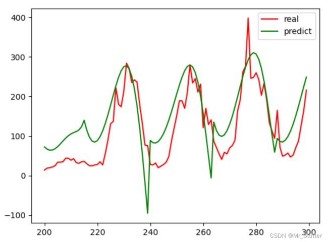
#可视化
start, end = 200, 300
x_range = np.arange(start, end)#展示一段内的拟合效果
plt.plot(x_range, y[start:end], 'r', label='real')#实际
plt.plot(x_range, y_predict[start:end], 'g', label='predict')#预测
plt.legend(loc='upper right')#图例
plt.show()

4、运行结果

---

总结

sklearn中，多项式回归利用sklearn.preprocessing模块使自变量构造成非线性特征，再调用线性回归模型将因变量与非线性特征进行线性拟合；岭回归在多项式回归的基础上用岭回归拟合代替线性拟合。