手撕代码：VGG13实战CIFAR数据集，附：卷积神经网络CNN可视化学习

VGG13实战

VGG模型是2014年ILSVRC竞赛的第二名，第一名是GoogLeNet。但是VGG模型在多个迁移学习任务中的表现要优于googLeNet。而且，从图像中提取CNN特征，VGG模型是首选算法。
“VGG”代表了牛津大学的Oxford Visual Geometry Group
特点：

1. 小卷积核：作者将卷积核全部替换为3x3（极少用了1x1）；
2. 小池化核：相比AlexNet的3x3的池化核，VGG全部为2x2的池化核；
3. 层数更深特征图更宽：基于前两点外，由于卷积核专注于扩大通道数、池化专注于缩小宽和高，使得模型架构上更深更宽的同时，计算量的增加放缓；
4. 全连接转卷积：网络测试阶段将训练阶段的三个全连接替换为三个卷积，测试重用训练时的参数，使得测试得到的全卷积网络因为没有全连接的限制，因而可以接收任意宽或高为的输入。

引自百度百科：https://baike.baidu.com/item/VGG%20模型/22689655?fr=aladdin

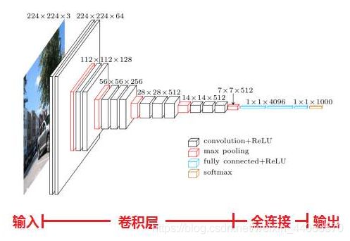
本次实战的代码是VGG13，即图中红色框部分的结构

代码如下

import  tensorflow as tf
from    tensorflow.keras import layers, optimizers, datasets, Sequential
import  os

os.environ['TF_CPP_MIN_LOG_LEVEL']='2'
tf.random.set_seed(2345)

conv_layers = [ # 5 units of conv + max pooling
    # unit 1   channel =64
    layers.Conv2D(64, kernel_size=[3, 3], padding="same", activation=tf.nn.relu),
    layers.Conv2D(64, kernel_size=[3, 3], padding="same", activation=tf.nn.relu),
    layers.MaxPool2D(pool_size=[2, 2], strides=2, padding='same'),

    # unit 2   channel =128
    layers.Conv2D(128, kernel_size=[3, 3], padding="same", activation=tf.nn.relu),
    layers.Conv2D(128, kernel_size=[3, 3], padding="same", activation=tf.nn.relu),
    layers.MaxPool2D(pool_size=[2, 2], strides=2, padding='same'),

    # unit 3   channel =256
    layers.Conv2D(256, kernel_size=[3, 3], padding="same", activation=tf.nn.relu),
    layers.Conv2D(256, kernel_size=[3, 3], padding="same", activation=tf.nn.relu),
    layers.MaxPool2D(pool_size=[2, 2], strides=2, padding='same'),

    # unit 4   channel =512
    layers.Conv2D(512, kernel_size=[3, 3], padding="same", activation=tf.nn.relu),
    layers.Conv2D(512, kernel_size=[3, 3], padding="same", activation=tf.nn.relu),
    layers.MaxPool2D(pool_size=[2, 2], strides=2, padding='same'),

    # unit 5   channel =512
    layers.Conv2D(512, kernel_size=[3, 3], padding="same", activation=tf.nn.relu),
    layers.Conv2D(512, kernel_size=[3, 3], padding="same", activation=tf.nn.relu),
    layers.MaxPool2D(pool_size=[2, 2], strides=2, padding='same')

]



def preprocess(x, y):
    # [0~1]
    x = tf.cast(x, dtype=tf.float32) / 255.
    y = tf.cast(y, dtype=tf.int32)
    return x,y


(x,y), (x_test, y_test) = datasets.cifar100.load_data()
y = tf.squeeze(y, axis=1)            # 根据sample输出的格式squeeze多余维度
y_test = tf.squeeze(y_test, axis=1)
print(x.shape, y.shape, x_test.shape, y_test.shape)


train_db = tf.data.Dataset.from_tensor_slices((x,y))
train_db = train_db.shuffle(1000).map(preprocess).batch(128)

test_db = tf.data.Dataset.from_tensor_slices((x_test,y_test))
test_db = test_db.map(preprocess).batch(64)

# 测试sample的形状：(batchsize, h, w, channel)
sample = next(iter(train_db))
print('sample:', sample[0].shape, sample[1].shape,
      tf.reduce_min(sample[0]), tf.reduce_max(sample[0]))


def main():

    conv_net = Sequential(conv_layers)
    # # 查看输出格式 [b, 32, 32, 3] => [b, 1, 1, 512]
    # conv_net.build(input_shape=[None,32,32,3])
    # x = tf.random.normal([4,32,32,3])
    # out = conv_net(x)
    # print(out.shape)

    # 全连接层
    fc_net = Sequential([
        layers.Dense(256, activation=tf.nn.relu),
        layers.Dense(128, activation=tf.nn.relu),
        layers.Dense(100, activation=None),
    ])
    # 将网络分为两部分，第一部分的输出即位为第二部分的输入
    conv_net.build(input_shape=[None, 32, 32, 3])
    fc_net.build(input_shape=[None, 512])
    optimizer = optimizers.Adam(lr=1e-4)

    # 网络两部分的参数放在一起 “+”运作原理：[1, 2] + [3, 4] => [1, 2, 3, 4]
    variables = conv_net.trainable_variables + fc_net.trainable_variables

    for epoch in range(50):

        for step, (x,y) in enumerate(train_db):

            with tf.GradientTape() as tape:
                # [b, 32, 32, 3] => [b, 1, 1, 512]
                out = conv_net(x)
                # flatten, => [b, 512] 打平送入全连接层
                out = tf.reshape(out, [-1, 512])
                # [b, 512] => [b, 100]
                logits = fc_net(out)
                # [b] => [b, 100]
                y_onehot = tf.one_hot(y, depth=100)
                # compute loss
                loss = tf.losses.categorical_crossentropy(y_onehot, logits, from_logits=True)
                loss = tf.reduce_mean(loss)

            grads = tape.gradient(loss, variables)      # Variables处理在line83
            optimizer.apply_gradients(zip(grads, variables))

            if step %100 == 0:
                print(epoch, step, 'loss:', float(loss))


       # 测试部分
        total_num = 0
        total_correct = 0
        for x,y in test_db:

            out = conv_net(x)
            out = tf.reshape(out, [-1, 512])
            logits = fc_net(out)
            prob = tf.nn.softmax(logits, axis=1)
            pred = tf.argmax(prob, axis=1)
            pred = tf.cast(pred, dtype=tf.int32)

            correct = tf.cast(tf.equal(pred, y), dtype=tf.int32)
            correct = tf.reduce_sum(correct)

            total_num += x.shape[0]
            total_correct += int(correct)

        acc = total_correct / total_num
        print(epoch, 'acc:', acc)



if __name__ == '__main__':
    main()

卷积神经网络CNN可视化学习

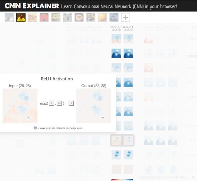
此外，分享一个可视化CNN的网站，用chrome打开哟！
https://poloclub.github.io/cnn-explainer/
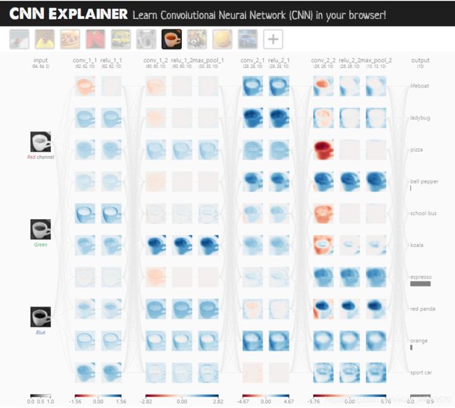点击每个环节可以查看具体的过程的可视化，太牛逼了！
卷积层

ReLU激活

SoftMax分类

还有很多可以探索的地方，太酷炫了！

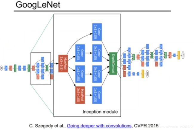
#GoogLeNet (Inception)简述
作为和VGG同时代的网络，在这里也放一张结构图以作对比。
GoogLeNet有Inception V1~V4四个版本的进化，
后来还融入SelectiveSearch等技术实现了目标检测任务，和FCN等技术融合实现图像分割等…
等待更进一步的学习再来补充吧。