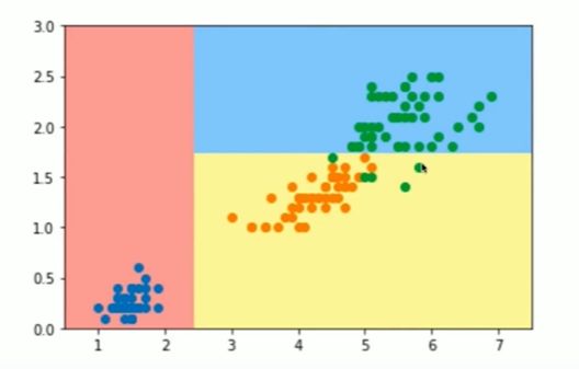
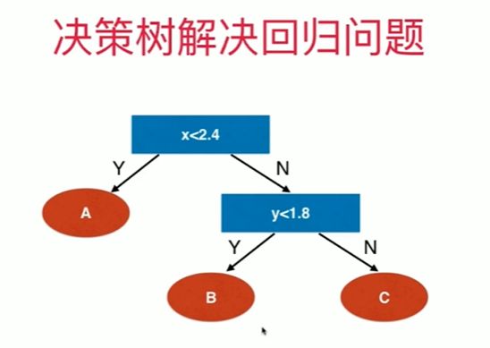
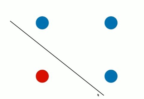
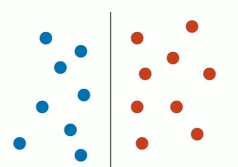
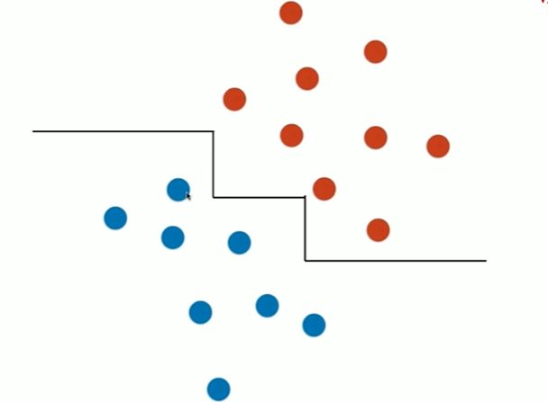
12-1 什么是决策树


Notbook 示例
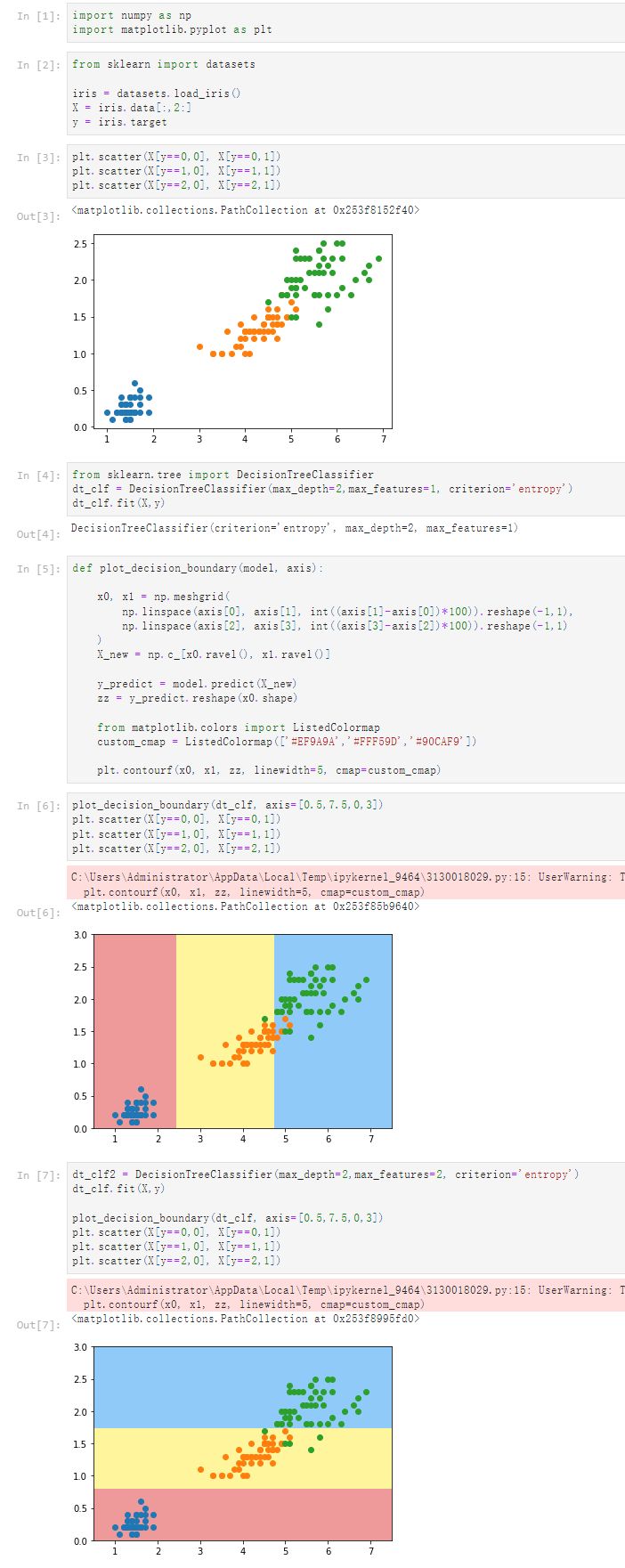
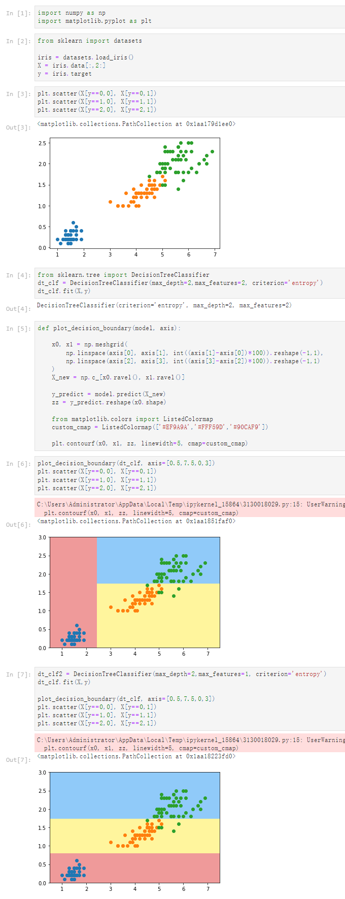
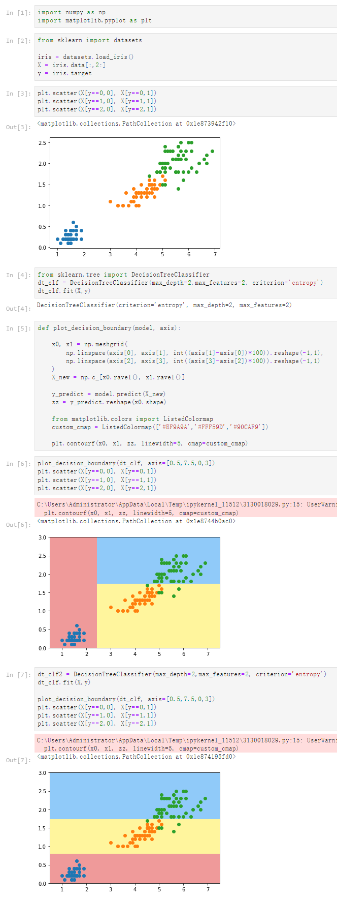
疑问:改变max_features 的值,图像具有一定随机性
notbook 源码
[1]
import numpy as np
import matplotlib.pyplot as plt
[2]
from sklearn import datasets

iris = datasets.load_iris()
X = iris.data[:,2:]
y = iris.target
[3]
plt.scatter(X[y==0,0], X[y==0,1])
plt.scatter(X[y==1,0], X[y==1,1])
plt.scatter(X[y==2,0], X[y==2,1])


[4]
from sklearn.tree import DecisionTreeClassifier
dt_clf = DecisionTreeClassifier(max_depth=2,max_features=2, criterion='entropy')
dt_clf.fit(X,y)
DecisionTreeClassifier(criterion='entropy', max_depth=2, max_features=2)
[5]
def plot_decision_boundary(model, axis):

    x0, x1 = np.meshgrid(
        np.linspace(axis[0], axis[1], int((axis[1]-axis[0])*100)).reshape(-1,1),
        np.linspace(axis[2], axis[3], int((axis[3]-axis[2])*100)).reshape(-1,1)
    )
    X_new = np.c_[x0.ravel(), x1.ravel()]

    y_predict = model.predict(X_new)
    zz = y_predict.reshape(x0.shape)

    from matplotlib.colors import ListedColormap
    custom_cmap = ListedColormap(['#EF9A9A','#FFF59D','#90CAF9'])

    plt.contourf(x0, x1, zz, linewidth=5, cmap=custom_cmap)
[6]
plot_decision_boundary(dt_clf, axis=[0.5,7.5,0,3])
plt.scatter(X[y==0,0], X[y==0,1])
plt.scatter(X[y==1,0], X[y==1,1])
plt.scatter(X[y==2,0], X[y==2,1])
C:\Users\Administrator\AppData\Local\Temp\ipykernel_15136\3130018029.py:15: UserWarning: The following kwargs were not used by contour: 'linewidth'
  plt.contourf(x0, x1, zz, linewidth=5, cmap=custom_cmap)


[7]
dt_clf2 = DecisionTreeClassifier(max_depth=2,max_features=1, criterion='entropy')
dt_clf.fit(X,y)

plot_decision_boundary(dt_clf, axis=[0.5,7.5,0,3])
plt.scatter(X[y==0,0], X[y==0,1])
plt.scatter(X[y==1,0], X[y==1,1])
plt.scatter(X[y==2,0], X[y==2,1])
C:\Users\Administrator\AppData\Local\Temp\ipykernel_15136\3130018029.py:15: UserWarning: The following kwargs were not used by contour: 'linewidth'
  plt.contourf(x0, x1, zz, linewidth=5, cmap=custom_cmap)
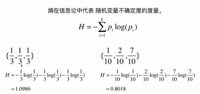
12-2 信息熵


Notbook 示例

Notbook 源码
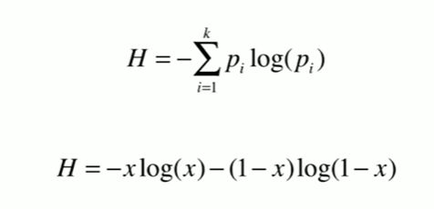
信息熵
[2]
import numpy as np
import matplotlib.pyplot as plt
[6]
def entropy(p):
return -p * np.log(p) - (1-p) * np.log(1-p)
[7]
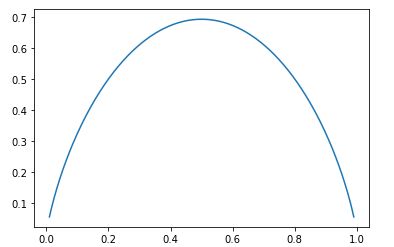
X = np.linspace(0.01, 0.99, 200)
[8]
plt.plot(X,entropy(X))
[]
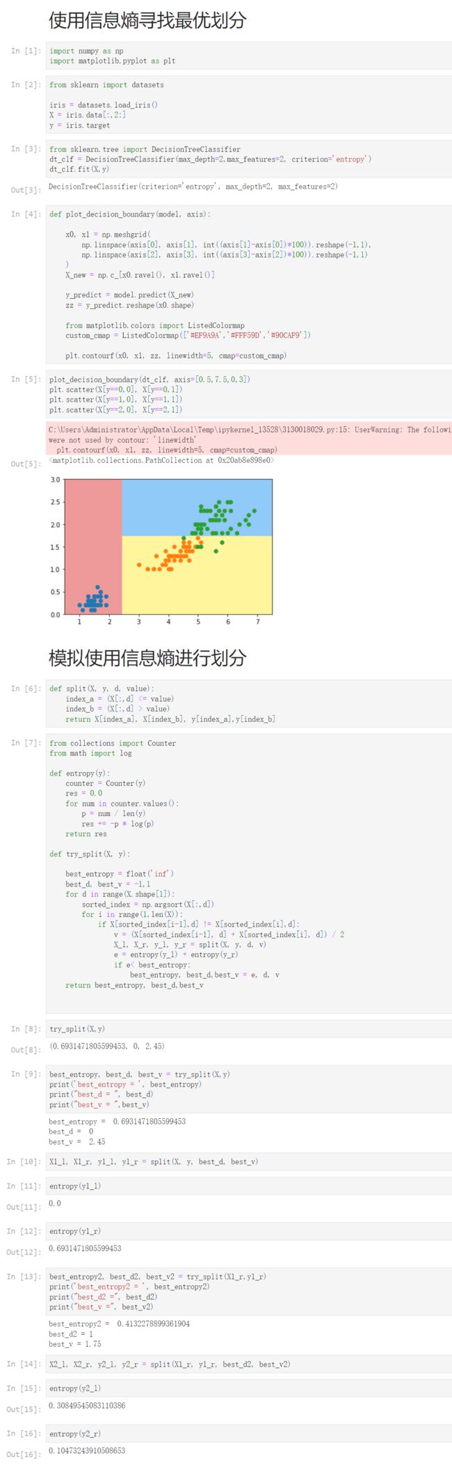
12-3 使用信息熵寻找最优划分
Notbook 示例
Notbook 源码
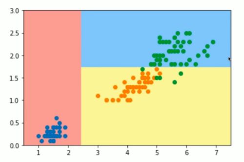
使用信息熵寻找最优划分
[1]
import numpy as np
import matplotlib.pyplot as plt
[2]
from sklearn import datasets

iris = datasets.load_iris()
X = iris.data[:,2:]
y = iris.target
[3]
from sklearn.tree import DecisionTreeClassifier
dt_clf = DecisionTreeClassifier(max_depth=2,max_features=2, criterion='entropy')
dt_clf.fit(X,y)
DecisionTreeClassifier(criterion='entropy', max_depth=2, max_features=2)
[4]
def plot_decision_boundary(model, axis):

    x0, x1 = np.meshgrid(
        np.linspace(axis[0], axis[1], int((axis[1]-axis[0])*100)).reshape(-1,1),
        np.linspace(axis[2], axis[3], int((axis[3]-axis[2])*100)).reshape(-1,1)
    )
    X_new = np.c_[x0.ravel(), x1.ravel()]

    y_predict = model.predict(X_new)
    zz = y_predict.reshape(x0.shape)

    from matplotlib.colors import ListedColormap
    custom_cmap = ListedColormap(['#EF9A9A','#FFF59D','#90CAF9'])

    plt.contourf(x0, x1, zz, linewidth=5, cmap=custom_cmap)
[5]
plot_decision_boundary(dt_clf, axis=[0.5,7.5,0,3])
plt.scatter(X[y==0,0], X[y==0,1])
plt.scatter(X[y==1,0], X[y==1,1])
plt.scatter(X[y==2,0], X[y==2,1])
C:\Users\Administrator\AppData\Local\Temp\ipykernel_13528\3130018029.py:15: UserWarning: The following kwargs were not used by contour: 'linewidth'
  plt.contourf(x0, x1, zz, linewidth=5, cmap=custom_cmap)


模拟使用信息熵进行划分
[6]
def split(X, y, d, value):
    index_a = (X[:,d] <= value)
    index_b = (X[:,d] > value)
    return X[index_a], X[index_b], y[index_a],y[index_b]
[7]
from collections import Counter
from math import log

def entropy(y):
    counter = Counter(y)
    res = 0.0
    for num in counter.values():
        p = num / len(y)
        res += -p * log(p)
    return res

def try_split(X, y):

    best_entropy = float('inf')
    best_d, best_v = -1,1
    for d in range(X.shape[1]):
        sorted_index = np.argsort(X[:,d])
        for i in range(1,len(X)):
            if X[sorted_index[i-1],d] != X[sorted_index[i],d]:
                v = (X[sorted_index[i-1], d] + X[sorted_index[i], d]) / 2
                X_l, X_r, y_l, y_r = split(X, y, d, v)
                e = entropy(y_l) + entropy(y_r)
                if e< best_entropy:
                    best_entropy, best_d,best_v = e, d, v
    return best_entropy, best_d,best_v


[8]
try_split(X,y)
(0.6931471805599453, 0, 2.45)
[9]
best_entropy, best_d, best_v = try_split(X,y)
print('best_entropy = ', best_entropy)
print("best_d = ", best_d)
print("best_v = ",best_v)
best_entropy =  0.6931471805599453
best_d =  0
best_v =  2.45

[10]
X1_l, X1_r, y1_l, y1_r = split(X, y, best_d, best_v)
[11]
entropy(y1_l)
0.0
[12]
entropy(y1_r)
0.6931471805599453
[13]
best_entropy2, best_d2, best_v2 = try_split(X1_r,y1_r)
print('best_entropy2 = ', best_entropy2)
print("best_d2 =", best_d2)
print("best_v =", best_v2)
best_entropy2 =  0.4132278899361904
best_d2 = 1
best_v = 1.75

[14]
X2_l, X2_r, y2_l, y2_r = split(X1_r, y1_r, best_d2, best_v2)
[15]
entropy(y2_l)
0.30849545083110386
[16]
entropy(y2_r)
0.10473243910508653
12-4 基尼系数


Notbook 示例
Notbook 源码
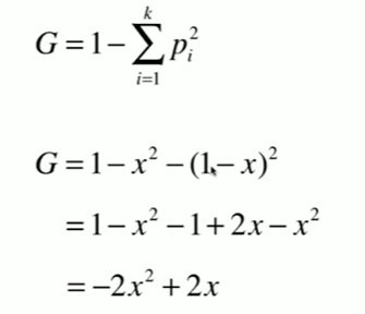
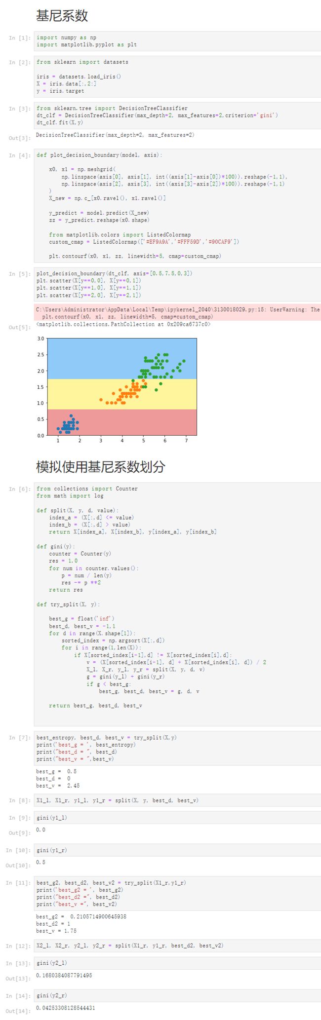
基尼系数
[1]
import numpy as np
import matplotlib.pyplot as plt
[2]
from sklearn import datasets

iris = datasets.load_iris()
X = iris.data[:,2:]
y = iris.target
[3]
from sklearn.tree import DecisionTreeClassifier
dt_clf = DecisionTreeClassifier(max_depth=2, max_features=2,criterion='gini')
dt_clf.fit(X,y)
DecisionTreeClassifier(max_depth=2, max_features=2)
[4]
def plot_decision_boundary(model, axis):

    x0, x1 = np.meshgrid(
        np.linspace(axis[0], axis[1], int((axis[1]-axis[0])*100)).reshape(-1,1),
        np.linspace(axis[2], axis[3], int((axis[3]-axis[2])*100)).reshape(-1,1)
    )
    X_new = np.c_[x0.ravel(), x1.ravel()]

    y_predict = model.predict(X_new)
    zz = y_predict.reshape(x0.shape)

    from matplotlib.colors import ListedColormap
    custom_cmap = ListedColormap(['#EF9A9A','#FFF59D','#90CAF9'])

    plt.contourf(x0, x1, zz, linewidth=5, cmap=custom_cmap)
[5]
plot_decision_boundary(dt_clf, axis=[0.5,7.5,0,3])
plt.scatter(X[y==0,0], X[y==0,1])
plt.scatter(X[y==1,0], X[y==1,1])
plt.scatter(X[y==2,0], X[y==2,1])
C:\Users\Administrator\AppData\Local\Temp\ipykernel_2040\3130018029.py:15: UserWarning: The following kwargs were not used by contour: 'linewidth'
  plt.contourf(x0, x1, zz, linewidth=5, cmap=custom_cmap)


模拟使用基尼系数划分
[6]
from collections import Counter
from math import log

def split(X, y, d, value):
    index_a = (X[:,d] <= value)
    index_b = (X[:,d] > value)
    return X[index_a], X[index_b], y[index_a], y[index_b]

def gini(y):
    counter = Counter(y)
    res = 1.0
    for num in counter.values():
        p = num / len(y)
        res -= p **2
    return res

def try_split(X, y):

    best_g = float('inf')
    best_d, best_v = -1,1
    for d in range(X.shape[1]):
        sorted_index = np.argsort(X[:,d])
        for i in range(1,len(X)):
            if X[sorted_index[i-1],d] != X[sorted_index[i],d]:
                v = (X[sorted_index[i-1], d] + X[sorted_index[i], d]) / 2
                X_l, X_r, y_l, y_r = split(X, y, d, v)
                g = gini(y_l) + gini(y_r)
                if g < best_g:
                    best_g, best_d, best_v = g, d, v

    return best_g, best_d, best_v


[7]
best_entropy, best_d, best_v = try_split(X,y)
print('best_g = ', best_entropy)
print("best_d = ", best_d)
print("best_v = ",best_v)
best_g =  0.5
best_d =  0
best_v =  2.45

[8]
X1_l, X1_r, y1_l, y1_r = split(X, y, best_d, best_v)
[9]
gini(y1_l)
0.0
[10]
gini(y1_r)
0.5
[11]
best_g2, best_d2, best_v2 = try_split(X1_r,y1_r)
print('best_g2 = ', best_g2)
print("best_d2 =", best_d2)
print("best_v =", best_v2)
best_g2 =  0.2105714900645938
best_d2 = 1
best_v = 1.75

[12]
X2_l, X2_r, y2_l, y2_r = split(X1_r, y1_r, best_d2, best_v2)
[13]
gini(y2_l)
0.1680384087791495
[14]
gini(y2_r)
0.04253308128544431
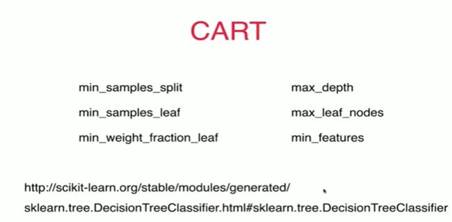
12-5 CART与决策树中的超参数


Notbook 示例
Notbook 源码
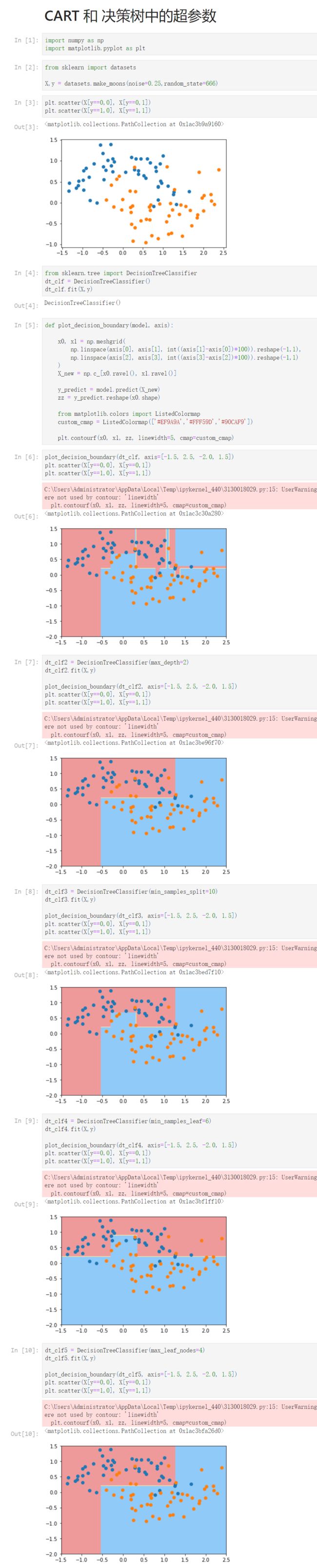
CART 和 决策树中的超参数
[1]
import numpy as np
import matplotlib.pyplot as plt
[2]
from sklearn import datasets

X,y = datasets.make_moons(noise=0.25,random_state=666)
[3]
plt.scatter(X[y==0,0], X[y==0,1])
plt.scatter(X[y==1,0], X[y==1,1])


[4]
from sklearn.tree import DecisionTreeClassifier
dt_clf = DecisionTreeClassifier()
dt_clf.fit(X,y)
DecisionTreeClassifier()
[5]
def plot_decision_boundary(model, axis):

    x0, x1 = np.meshgrid(
        np.linspace(axis[0], axis[1], int((axis[1]-axis[0])*100)).reshape(-1,1),
        np.linspace(axis[2], axis[3], int((axis[3]-axis[2])*100)).reshape(-1,1)
    )
    X_new = np.c_[x0.ravel(), x1.ravel()]

    y_predict = model.predict(X_new)
    zz = y_predict.reshape(x0.shape)

    from matplotlib.colors import ListedColormap
    custom_cmap = ListedColormap(['#EF9A9A','#FFF59D','#90CAF9'])

    plt.contourf(x0, x1, zz, linewidth=5, cmap=custom_cmap)
[6]
plot_decision_boundary(dt_clf, axis=[-1.5, 2.5, -2.0, 1.5])
plt.scatter(X[y==0,0], X[y==0,1])
plt.scatter(X[y==1,0], X[y==1,1])
C:\Users\Administrator\AppData\Local\Temp\ipykernel_440\3130018029.py:15: UserWarning: The following kwargs were not used by contour: 'linewidth'
  plt.contourf(x0, x1, zz, linewidth=5, cmap=custom_cmap)


[7]
dt_clf2 = DecisionTreeClassifier(max_depth=2)
dt_clf2.fit(X,y)

plot_decision_boundary(dt_clf2, axis=[-1.5, 2.5, -2.0, 1.5])
plt.scatter(X[y==0,0], X[y==0,1])
plt.scatter(X[y==1,0], X[y==1,1])
C:\Users\Administrator\AppData\Local\Temp\ipykernel_440\3130018029.py:15: UserWarning: The following kwargs were not used by contour: 'linewidth'
  plt.contourf(x0, x1, zz, linewidth=5, cmap=custom_cmap)


[8]
dt_clf3 = DecisionTreeClassifier(min_samples_split=10)
dt_clf3.fit(X,y)

plot_decision_boundary(dt_clf3, axis=[-1.5, 2.5, -2.0, 1.5])
plt.scatter(X[y==0,0], X[y==0,1])
plt.scatter(X[y==1,0], X[y==1,1])
C:\Users\Administrator\AppData\Local\Temp\ipykernel_440\3130018029.py:15: UserWarning: The following kwargs were not used by contour: 'linewidth'
  plt.contourf(x0, x1, zz, linewidth=5, cmap=custom_cmap)


[9]
dt_clf4 = DecisionTreeClassifier(min_samples_leaf=6)
dt_clf4.fit(X,y)

plot_decision_boundary(dt_clf4, axis=[-1.5, 2.5, -2.0, 1.5])
plt.scatter(X[y==0,0], X[y==0,1])
plt.scatter(X[y==1,0], X[y==1,1])
C:\Users\Administrator\AppData\Local\Temp\ipykernel_440\3130018029.py:15: UserWarning: The following kwargs were not used by contour: 'linewidth'
  plt.contourf(x0, x1, zz, linewidth=5, cmap=custom_cmap)


[10]
dt_clf5 = DecisionTreeClassifier(max_leaf_nodes=4)
dt_clf5.fit(X,y)

plot_decision_boundary(dt_clf5, axis=[-1.5, 2.5, -2.0, 1.5])
plt.scatter(X[y==0,0], X[y==0,1])
plt.scatter(X[y==1,0], X[y==1,1])
C:\Users\Administrator\AppData\Local\Temp\ipykernel_440\3130018029.py:15: UserWarning: The following kwargs were not used by contour: 'linewidth'
  plt.contourf(x0, x1, zz, linewidth=5, cmap=custom_cmap)
12-6 决策树解决回归问题


Notbook 示例
Notbook 源码
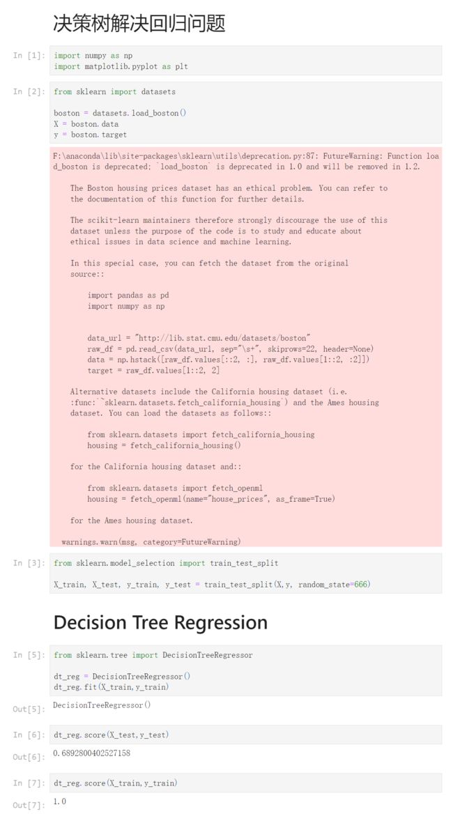
决策树解决回归问题
[1]
import numpy as np
import matplotlib.pyplot as plt
[2]
from sklearn import datasets

boston = datasets.load_boston()
X = boston.data
y = boston.target
F:\anaconda\lib\site-packages\sklearn\utils\deprecation.py:87: FutureWarning: Function load_boston is deprecated; `load_boston` is deprecated in 1.0 and will be removed in 1.2.

    The Boston housing prices dataset has an ethical problem. You can refer to
    the documentation of this function for further details.

    The scikit-learn maintainers therefore strongly discourage the use of this
    dataset unless the purpose of the code is to study and educate about
    ethical issues in data science and machine learning.

    In this special case, you can fetch the dataset from the original
    source::

        import pandas as pd
        import numpy as np


        data_url = "http://lib.stat.cmu.edu/datasets/boston"
        raw_df = pd.read_csv(data_url, sep="\s+", skiprows=22, header=None)
        data = np.hstack([raw_df.values[::2, :], raw_df.values[1::2, :2]])
        target = raw_df.values[1::2, 2]

    Alternative datasets include the California housing dataset (i.e.
    :func:`~sklearn.datasets.fetch_california_housing`) and the Ames housing
    dataset. You can load the datasets as follows::

        from sklearn.datasets import fetch_california_housing
        housing = fetch_california_housing()

    for the California housing dataset and::

        from sklearn.datasets import fetch_openml
        housing = fetch_openml(name="house_prices", as_frame=True)

    for the Ames housing dataset.

  warnings.warn(msg, category=FutureWarning)

[3]
from sklearn.model_selection import train_test_split

X_train, X_test, y_train, y_test = train_test_split(X,y, random_state=666)
Decision Tree Regression
[5]
from sklearn.tree import DecisionTreeRegressor

dt_reg = DecisionTreeRegressor()
dt_reg.fit(X_train,y_train)
DecisionTreeRegressor()
[6]
dt_reg.score(X_test,y_test)
0.6892800402527158
[7]
dt_reg.score(X_train,y_train)
1.0
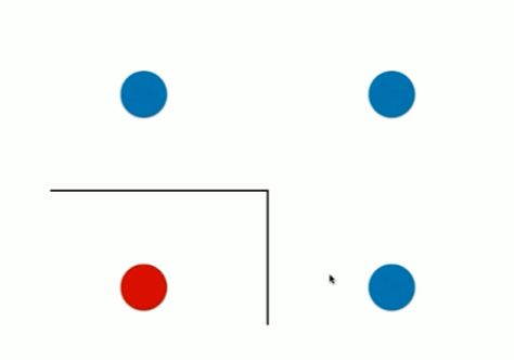
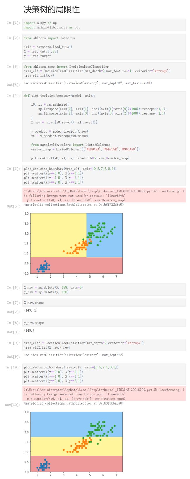
12-7 决策树的局限性


Notbook 示例
Notbook 源码
决策树的局限性
[1]
import numpy as np
import matplotlib.pyplot as plt
[2]
from sklearn import datasets

iris = datasets.load_iris()
X = iris.data[:,2:]
y = iris.target
[3]
from sklearn.tree import DecisionTreeClassifier
tree_clf = DecisionTreeClassifier(max_depth=2,max_features=1, criterion='entropy')
tree_clf.fit(X,y)
DecisionTreeClassifier(criterion='entropy', max_depth=2, max_features=1)
[4]
def plot_decision_boundary(model, axis):

    x0, x1 = np.meshgrid(
        np.linspace(axis[0], axis[1], int((axis[1]-axis[0])*100)).reshape(-1,1),
        np.linspace(axis[2], axis[3], int((axis[3]-axis[2])*100)).reshape(-1,1)
    )
    X_new = np.c_[x0.ravel(), x1.ravel()]

    y_predict = model.predict(X_new)
    zz = y_predict.reshape(x0.shape)

    from matplotlib.colors import ListedColormap
    custom_cmap = ListedColormap(['#EF9A9A','#FFF59D','#90CAF9'])

    plt.contourf(x0, x1, zz, linewidth=5, cmap=custom_cmap)
[5]
plot_decision_boundary(tree_clf, axis=[0.5,7.5,0,3])
plt.scatter(X[y==0,0], X[y==0,1])
plt.scatter(X[y==1,0], X[y==1,1])
plt.scatter(X[y==2,0], X[y==2,1])
C:\Users\Administrator\AppData\Local\Temp\ipykernel_17836\3130018029.py:15: UserWarning: The following kwargs were not used by contour: 'linewidth'
  plt.contourf(x0, x1, zz, linewidth=5, cmap=custom_cmap)


[6]
X_new = np.delete(X, 138, axis=0)
y_new = np.delete(y, 138)
[7]
X_new.shape
(149, 2)
[8]
y_new.shape
(149,)
[9]
tree_clf2 = DecisionTreeClassifier(max_depth=2,criterion='entropy')
tree_clf2.fit(X_new,y_new)
DecisionTreeClassifier(criterion='entropy', max_depth=2)
[10]
plot_decision_boundary(tree_clf2, axis=[0.5,7.5,0,3])
plt.scatter(X[y==0,0], X[y==0,1])
plt.scatter(X[y==1,0], X[y==1,1])
plt.scatter(X[y==2,0], X[y==2,1])
C:\Users\Administrator\AppData\Local\Temp\ipykernel_17836\3130018029.py:15: UserWarning: The following kwargs were not used by contour: 'linewidth'
  plt.contourf(x0, x1, zz, linewidth=5, cmap=custom_cmap)