神经网络模型中class的forward函数何时调用_总结深度学习PyTorch神经网络箱使用...
↑ 点击 蓝字 关注极市平台 来源丨计算机视觉联盟 编辑丨极市平台
 数据加载DataLoader中
把输入数据传入神经网络Net实例化对象model中,自行执行forward函数,得到out输出值,然后用out与标记lable计算损失值Loss
缺省的情况下梯度是累加的,在梯度反向传播前,需要清零梯度
基于当前梯度更新参数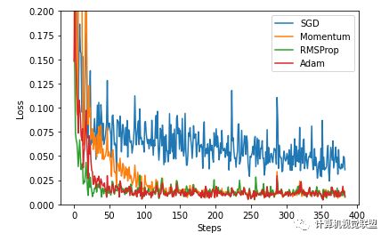
 添加极市小助手微信(ID : cvmart2),备注:姓名-学校/公司-研究方向-城市(如:小极-北大-目标检测-深圳),即可申请加入极市目标检测/图像分割/工业检测/人脸/医学影像/3D/SLAM/自动驾驶/超分辨率/姿态估计/ReID/GAN/图像增强/OCR/视频理解等技术交流群:每月大咖直播分享、真实项目需求对接、求职内推、算法竞赛、干货资讯汇总、与 10000+来自港科大、北大、清华、中科院、CMU、腾讯、百度等名校名企视觉开发者互动交流~
  △长按添加极市小助手
  △长按关注极市平台,获取 最新CV干货 觉得有用麻烦给个在看啦~
极市导读
本文介绍了Pytorch神经网络箱的使用,包括核心组件、神经网络实例、构建方法、优化器比较等内容,非常全面。>>加入极市CV技术交流群,走在计算机视觉的最前沿
1 神经网络核心组件
核心组件包括:层:神经网络的基本结构,将输入张量转换为输出张量
模型:层构成的网络
损失函数:参数学习的目标函数,通过最小化损失函数来学习各种参数
优化器:如何是损失函数最小
2 神经网络实例
如果初学者,建议直接看3,避免运行结果有误。
神经网络工具及相互关系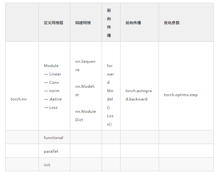
2.1 背景说明
如何利用神经网络完成对手些数字进行识别? 使用Pytorch内置函数mnist下载数据 利用torchvision对数据进行预处理,调用torch.utils建立一个数据迭代器 可视化源数据 利用nn工具箱构建神经网络模型 实例化模型,定义损失函数及优化器 训练模型 可视化结果 使用2个隐藏层,每层激活函数为ReLU,最后使用torch.max(out,1)找出张量out最大值对索引作为预测值
2.2 准备数据
##(1)导入必要的模块import numpy as npimport torch# 导入内置的 mnist数据from torchvision.datasets import mnist# 导入预处理模块import torchvision.transforms as transformsfrom torch.utils.data import DataLoader# 导入nn及优化器import torch.nn.functional as Fimport torch.optim as optimfrom torch import nn## (2) 定义一些超参数
train_batch_size = 64
test_batch_size = 128
learning_rate = 0.01
num_epoches = 20
lr = 0.01
momentum = 0.5## (3) 下载数据并对数据进行预处理# 定义预处理函数,这些预处理依次放在Compose函数中
transform = transforms.Compose([transforms.ToTensor(),transforms.Normalize([0.5],[0.5])])# 下载数据,并对数据进行预处理
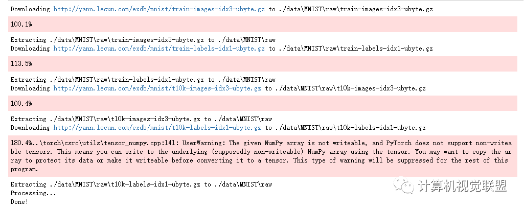
train_dataset = mnist.MNIST('./data', train=True, transform=transform, download=True)
test_dataset = mnist.MNIST('./data', train=False, transform=transform)# dataloader是一个可迭代的对象,可以使用迭代器一样使用
train_loader = DataLoader(train_dataset, batch_size=train_batch_size, shuffle=True)
test_loader = DataLoader(test_dataset, batch_size=test_batch_size, shuffle=False)2.3 可视化数据源
import matplotlib.pyplot as plt
%matplotlib inline
examples = enumerate(test_loader)
batch_idx, (example_data, example_targets) = next(examples)
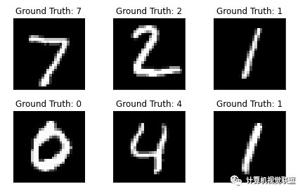
fig = plt.figure()for i in range(6):
plt.subplot(2,3,i+1)
plt.tight_layout()
plt.imshow(example_data[i][0], cmap='gray', interpolation='none')
plt.title("Ground Truth: {}".format(example_targets[i]))
plt.xticks([])
plt.yticks([])2.4 构建模型
## (1)构建网络
class Net(nn.Module):
    """
    使用sequential构建网络,Sequential()函数功能是将网络的层组合一起
    """
    def __init__(self, in_dim, n_hidden_1, n_hidden_2, out_dim):
        super(Net, self).__init__()
        self.layer1 = nn.Sequential(nn.Linear(in_dim, n_hidden_1),nn.BatchNorm1d(n_hidden_1))
        self.layer2 = nn.Sequential(nn.Linear(n_hidden_1, n_hidden_2),nn.BatchNorm1d(n_hidden_2))
        self.layer3 = nn.Sequential(nn.Linear(n_hidden_2, out_dim))
    def forward(self, x):
        x = F.relu(self.layer1(x))
        x = F.relu(self.layer2(x))
        x = self.layer3(x)
        return x
## (2)实例化网络
# 检测是否有GPU,有就用,没有就用CPU
device = torch.device("cuda:0" if torch.cuda.if_available else "cpu")
# 实例化网络
model = Net(28*28, 300, 100, 10)
model.to(device)
# 定义损失函数和优化器
criterion = nn.CrossEntropyLoss()
optimizer = optim.SGD(model.parameters(), lr=lr, momentum=momentum)
2.5 训练模型
## 训练模型
# 开始训练
losses = []
acces = []
eval_losses = []
eval_acces = []
print("开始循环,请耐心等待.....")
for epoch in range(num_epoches):
    train_loss = 0
    train_acc = 0
    model.train()
    # 动态修改参数学习率
    if epoch%5==0:
        optimizer.param_groups[0]['lr']*=0.1
    for img, label in train_loader:
        img=img.to(device)
        label = label.to(device)
        img = img.view(img.size(0), -1)
        # 向前传播
        out = model(img)
        loss = criterion(out, label)
        # 反向传播
        optimizer.zero_grad()
        loss.backward()
        optimizer.step()
        # 记录误差
        train_loss += loss.item()
        # 计算分类的准确率
        _, pred = out.max(1)
        num_correct = (pred == label).sum().item()
        acc = num_correct / img.shape[0]
        train_acc +=acc
    print("第一个循环结束,继续耐心等待....")
    losses.append(train_loss / len(train_loader))
    acces.append(train_acc / len(train_loader))
    # 在测试集上检验效果
    eval_loss = 0
    eval_acc = 0
    # 将模型改为预测模式
    model.eval()
    for img, label in test_loader:
        img=img.to(device)
        label=label.to(device)
        img=img.view(img.size(0),-1)
        out = model(img)
        loss = criterion(out, label)
        # 记录误差
        eval_loss += loss.item()
        # 记录准确率
        _, pred = out.max(1)
        num_correct = (pred == label).sum().item()
        acc = num_correct / img.shape[0]
        eval_acc +=acc
    print("第二个循环结束,准备结束")
    eval_losses.append(eval_loss / len(test_loader))
    eval_acces.append(eval_acc / len(test_loader))
print('epoch: {}, Train Loss: {:.4f}, Train Acc: {:.4f}, Test Loss: {:.4f}, Test Acc: {:.4f}'.format(epoch, train_loss / len(train_loader), train_acc / len(train_loader), eval_loss / len(test_loader), eval_acc / len(test_loader)))## 可视化训练结果
plt.title('trainloss')
plt.plot(np.arange(len(losses)), losses)
plt.legend(['Train Loss'], loc='upper right')
print("开始循环,请耐心等待.....")3 全连接神经网络进行MNIST识别
3.1 数据
import numpy as npimport torchfrom torchvision.datasets import mnistfrom torch import nnfrom torch.autograd import Variabledef data_tf(x):
x = np.array(x, dtype="float32")/255
x = (x-0.5)/0.5
x = x.reshape((-1)) # 这里是为了变为1行,然后m列
x = torch.from_numpy(x)
return x
# 下载数据集,有的话就不下载了
train_set = mnist.MNIST("./data",train=True, transform=data_tf, download=False)
test_set = mnist.MNIST("./data",train=False, transform=data_tf, download=False)
a, a_label = train_set[0]
print(a.shape)
print(a_label)3.2 可视化数据
import matplotlib.pyplot as plt
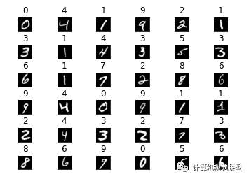
for i in range(1, 37):
plt.subplot(6,6,i)
plt.xticks([]) # 不显示坐标系
plt.yticks([])
plt.imshow(train_set.data[i].numpy(), cmap="gray")
plt.title("%i" % train_set.targets[i])
plt.subplots_adjust(wspace = 0 , hspace = 1) # 调整
plt.show()from torch.utils.data import DataLoader
train_data = DataLoader(train_set, batch_size=64, shuffle= True)
test_data = DataLoader(test_set, batch_size=128, shuffle=False)
a, a_label = next(iter(train_data))
print(a.shape)
print(a_label.shape)3.3 定义神经网络
神经网络一共四层net = nn.Sequential( nn.Linear(784, 400),
nn.ReLU(),
nn.Linear(400, 200),
nn.ReLU(),
nn.Linear(200, 100),
nn.ReLU(),
nn.Linear(100,10),
nn.ReLU()
)if torch.cuda.is_available():
net = net.cuda()criterion = nn.CrossEntropyLoss()
optimizer = torch.optim.SGD(net.parameters(), 1e-1)3.4 训练
losses = []
acces  = []
eval_losses = []
eval_acces  = []
# 一共训练20次
for e in range(20):
    train_loss = 0
    train_acc = 0
    net.train()
    for im, label in train_data:
        if torch.cuda.is_available():
            im = Variable(im).cuda()
            label = Variable(label).cuda()
        else:
            im = Variable(im)
            label =Variable(label)
        # 前向传播
        out = net(im)
        loss = criterion(out, label)
        # 反向传播
        optimizer.zero_grad()
        loss.backward()
        optimizer.step()
        # 误差
        train_loss += loss.item()
        #计算分类的准确率
        # max函数参数1表示按行取最大值,第一个返回值是值,第二个返回值是下标
        # pred是一个固定1*64的向量
        _,pred = out.max(1)
        num_correct = (pred==label).sum().item()
        acc = num_correct/im.shape[0]
        train_acc += acc
    # 此时一轮训练以及完了
    losses.append(train_loss/len(train_data))
    acces.append(train_acc/len(train_data))
    # 在测试集上检验效果
    eval_loss = 0
    eval_acc = 0
    net.eval()
    for im, label in test_data:
        if torch.cuda.is_available():
            im = Variable(im).cuda()
            label = Variable(label).cuda()
        else:
            im = Variable(im)
            label =Variable(label)
        # 前向传播
        out = net(im)
        # 计算误差
        loss = criterion(out, label)
        eval_loss += loss.item()
        # 计算准确率
        _,pred = out.max(1)
        num_correct = (pred==label).sum().item()
        acc = num_correct/im.shape[0]
        eval_acc += acc
    eval_losses.append(eval_loss/len(test_data))
    eval_acces.append(eval_acc/len(test_data))
    print('epoch: {}, Train Loss: {:.6f}, Train Acc: {:.6f}, Eval Loss: {:.6f}, Eval Acc: {:.6f}'.format(e, train_loss / len(train_data), train_acc / len(train_data), eval_loss / len(test_data), eval_acc / len(test_data)))
3.5 展示
%matplotlib inline
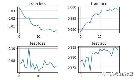
plt.subplot(2, 2, 1)
plt.title("train loss")
plt.plot(np.arange(len(losses)), losses)
plt.grid()
plt.subplot(2, 2, 2)
plt.title("train acc")
plt.plot(np.arange(len(acces)), acces)
plt.grid()
plt.subplot(2, 2, 3)
plt.title("test loss")
plt.plot(np.arange(len(eval_losses)), eval_losses)
plt.grid()
plt.subplot(2, 2, 4)
plt.title("test acc")
plt.plot(np.arange(len(eval_acces)), eval_acces)
plt.grid()
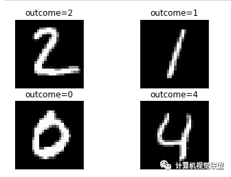
plt.subplots_adjust(wspace =0.5, hspace =0.5)for i in range(1, 5):
im = test_set.data[i]
label = test_set.targets[i]
plt.subplot(2, 2, i)
plt.imshow(im.numpy(), cmap="gray")
plt.xticks([])
plt.yticks([])
im = data_tf(im)
im = Variable(im).cuda()
out = net(im)
_, pred = out.max(0)
plt.title("outcome=%i" % pred.item())
plt.show()4 如何构建神经网络?
搭建神经网络主要包含:选择网络层,构建网络,选择损失和优化器。
nn工具箱可直接引用:全连接层,卷积层,循环层,正则化层,激活层。4.1 构建网络层
torch.nn.Sequential() 构建网络层 每层的编码是默认的数字,不易区分; 如果想对每层定义一个名称:可以在Sequential基础上通过add_module()添加每一层,并且为每一层增加一个单独的名字
通过字典的形式添加每一层,设置单独的层名称
class Net(torch.nn.Module):def __init__(self):
        super(Net4, self).__init__()
        self.conv = torch.nn.Sequential(
            OrderedDict(
                [
                    ("conv1", torch.nn.Conv2d(3, 32, 3, 1, 1)),
                    ("relu1", torch.nn.ReLU()),
                    ("pool", torch.nn.MaxPool2d(2))
                ]
            ))
        self.dense = torch.nn.Sequential(
            orderedDict([
            ("dense1", torch.nn.Linear(32*3*3,128)),
            ("relu2", torch.nn.ReLU()),
            ("dense2", torch.nn.Linear(128,10))
            ])
        )
4.2 前向、反向传播
forward函数的任务需要把输入层、网络层、输出层链接起来,实现信息的前向传导 让损失函数调用backward()即可4.3 训练模型
调用训练模型model.train(),会把所有module设置为训练模式; 测试验证阶段,使用model.eval(),会把所有training属性设置为False5 神经网络工具箱nn
nn工具箱有两个重要模块:nn.Model和nn.functinal 5.1 nn.Module 继承nn.Module,生成自己的网络层 采用class Net(torch.nn.Module),这些层都是子类 命名规则:nn.Xxx(第一个是大写):nn.Linear、nn.Conv2d、nn.CrossEntropyLoss5.2 nn.functional
命名规则:nn.functional.xxx 与nn.Module有相似,但两者也有具体差别: (1)nn.Xxx继承于 nn.Module,nn.Xxx需要先实例化并传入参数,以函数调用的方式调用实例化对象传入输入数据。能够很好地与nn.Sequential结合使用,而nn.functional.xxx无法结合 (2)nn.Xxx不需要定义和管理weight、bias参数,nn.functianal需要自己定义weight、bias参数,每次调用都要手动传入,不利于代码复用 (3)Dropout在训练和测试阶段有区别,nn.Xxx在调用model.eval()之后,自动实现状态的转换,而使用nn.functional.xxx却无此功能 有学习参数的用nn.Xxx;没有学习参数的用nn.functional或nn.Xxx6 优化器
Pytorch常用的优化算法封装在torch.optim里面 优化方法都是继承了基类optim.Optimizer,实现了优化步骤 随机梯度下降SGD就是最普通的优化器 使用优化器的一般步骤: (1)建立优化器实例 导入optim模块,实例化SGD优化器,这列使用动量参数momentum,是SGD的改良版import torch.optim as optim
optimizer = optimSGD(model.parameters(), lr=lr, momentum=momentum)把输入数据传入神经网络Net实例化对象model中,自行执行forward函数,得到out输出值,然后用out与标记lable计算损失值Loss
out = model(img)
loss = criterion(out, label)缺省的情况下梯度是累加的,在梯度反向传播前,需要清零梯度
opyimizer.zero_grad()loss.backward()基于当前梯度更新参数
optimizer.step()7 动态修改学习率参数
可以修改optimizer.param_groups 或者 新建 optimizer 注意:新建的optimizer虽然很简单轻便,但是新建的会有震荡 optimizer.param_groups- 长度1的list
- optimizer.param_groups[0]长度为6的字典,包括权重、lr、momentum等
for epoch in range(num_epoches):## 动态修改参数学习率if epoch%5==0
        optimizer.param_groups[0]['lr']*=0.1
        print(optimizer.param_groups[0]['lr'])for img, label in train_loader:
8 优化器的比较
各种优化器都有适应的场景 不过自适应优化器比较受欢迎## (1)导入需要的模块import torchimport torch.utils.data as Dataimport torch.nn.functional as Fimport matplotlib.pyplot as plt
%matplotlib inline#超参数
LR = 0.01
BATCH_SIZE =32
EPOCH =12## (2)生成数据# 生成训练数据# torch.unsqueeze()作用是将一维变二维,torch只能处理二维数据
x = torch.unsqueeze(torch.linspace(-1, 1, 1000), dim=1)# 0.1 * torch.normal(x.size()) 增加噪声
y = x.pow(2) + 0.1 * torch.normal(torch.zeros(*x.size()))
torch_dataset = Data.TensorDataset(x,y)# 一个代批量的生成器
loader = Data.DataLoader(dataset=torch_dataset, batch_size=BATCH_SIZE, shuffle=True)## (3)构建神经网络class Net(torch.nn.Module):# 初始化def __init__(self):
super(Net, self).__init__()
self.hidden = torch.nn.Linear(1, 20)
self.predict = torch.nn.Linear(20, 1)# 向前传递def forward(self, x):
x = F.relu(self.hidden(x))
x = self.predict(x)return x## (4)使用多种优化器
net_SGD = Net()
net_Momentum = Net()
net_RMSProp = Net()
net_Adam = Net()
nets = [net_SGD, net_Momentum, net_RMSProp, net_Adam]
opt_SGD =torch.optim.SGD(net_SGD.parameters(), lr=LR)
opt_Momentum =torch.optim.SGD(net_Momentum.parameters(), lr=LR, momentum = 0.9)
opt_RMSProp =torch.optim.RMSprop(net_RMSProp.parameters(), lr=LR, alpha = 0.9)
opt_Adam =torch.optim.Adam(net_Adam.parameters(), lr=LR, betas=(0.9, 0.99))
optimizers = [opt_SGD, opt_Momentum, opt_RMSProp, opt_Adam]## (5)训练模型
loss_func = torch.nn.MSELoss()
loss_his = [[], [], [], []]for epoch in range(EPOCH):for step, (batch_x, batch_y) in enumerate(loader):for net, opt, l_his in zip(nets, optimizers, loss_his):
output = net(batch_x)
loss = loss_func(output, batch_y)
opt.zero_grad()
loss.backward()
opt.step()
l_his.append(loss.data.numpy())
labels = ['SGD', 'Momentum', 'RMSProp', 'Adam']## (6)可视化结果for i, l_his in enumerate(loss_his):
plt.plot(l_his, label=labels[i])
plt.legend(loc='best')
plt.xlabel('Steps')
plt.ylabel('Loss')
plt.ylim((0, 0.2))
plt.show()推荐阅读
基于Pytorch的动态卷积复现
当代研究生应当掌握的5种Pytorch并行训练方法(单机多卡)
综述|核心开发者全面解读Pytorch内部机制
添加极市小助手微信(ID : cvmart2),备注:姓名-学校/公司-研究方向-城市(如:小极-北大-目标检测-深圳),即可申请加入极市目标检测/图像分割/工业检测/人脸/医学影像/3D/SLAM/自动驾驶/超分辨率/姿态估计/ReID/GAN/图像增强/OCR/视频理解等技术交流群:每月大咖直播分享、真实项目需求对接、求职内推、算法竞赛、干货资讯汇总、与 10000+来自港科大、北大、清华、中科院、CMU、腾讯、百度等名校名企视觉开发者互动交流~ △长按添加极市小助手 △长按关注极市平台,获取 最新CV干货 觉得有用麻烦给个在看啦~