Ceres Tutotial（1） —— 编程应用基础

重要的Reference

• ceres 官方 tutorial
• 文章中的代码参考

1 install

# install dependencies
sudo apt-get install liblapack-dev libsuitesparse-dev libcxsparse3.1.4 libgflags-dev libgoogle-glog-dev libgtest-dev

# clone
git clone https://github.com/ceres-solver/ceres-solver.git

# build
cd ceres-solver
mkdir build
cmake ..
make
sudo make install

2 最小二乘问题的ceres表示

ceres要求解的问题是最小二乘问题。一般的最小二乘问题定义如下：
$$\begin{array}{cl}{\min }_{\mathbf{x}}& \frac{1}{2}{\sum }_i{\rho }_i\left({\Vert f_i\left(x_{i_1},\dots ,x_{i_k}\right)\Vert }^2\right)\\ \text{ s.t. }& l_j\le x_j\le u_j\end{array}$$

• 整个表达式称为ResidualBlock
• ${\rho }_i$是LossFucntion，也叫鲁棒核函数，主要是为了应对outliers
• $\left[x_{i_1},\dots ,x_{i_k}\right]$ ParameterBlock
• $f_i$ 称为CostFunction,通过调用这个函数可以计算残差residual

一个入门的Demo

#include "ceres/ceres.h"
#include "glog/logging.h"

using ceres::AutoDiffCostFunction;
using ceres::CostFunction;
using ceres::Problem;
using ceres::Solver;
using ceres::Solve;

// A templated cost functor that implements the residual r = 10 -
// x. The method operator() is templated so that we can then use an
// automatic differentiation wrapper around it to generate its
// derivatives.
// 定义cost function的调用函数接口，是一个仿函数functor
// ceres::CostFunction通过这个函数来计算残差Residual
struct CostFunctor {
    template<typename T>
    bool operator()(const T *const x, T *residual) const {
        residual[0] = 10.0 - x[0];
        return true;
    }
};

int main(int argc, char **argv) {
    google::InitGoogleLogging(argv[0]);

    // The variable to solve for with its initial value. It will be
    // mutated in place by the solver.
    double x = 0.5;
    const double initial_x = x;

    // 1. 构建求解问题
    Problem problem;

    // Set up the only cost function (also known as residual). This uses
    // auto-differentiation to obtain the derivative (jacobian).
    // 2. 定义cost function，此处是使用自动求导
    CostFunction *cost_function = new AutoDiffCostFunction<CostFunctor, 1, 1>(new CostFunctor);

    // 3. 添加残差块，具体包括3个项目
    // CostFunction, LossFunction, ParameterBlock
    problem.AddResidualBlock(cost_function, NULL, &x);

    // 4. 进行求解设置，打印输出
    Solver::Options options;
    options.minimizer_progress_to_stdout = true;
    Solver::Summary summary;
    Solve(options, &problem, &summary);

    std::cout << summary.BriefReport() << "\n";
    std::cout << "x : " << initial_x
              << " -> " << x << "\n";
    return 0;
}

3 求导

最小二乘问题描述

3.1 自动求导

上一个入门的例子，展示了如何利用ceres的自动求导

// 定义一个是模板成员函数的仿函数
struct CostFunctor {
    template<typename T>
    bool operator()(const T *const x, T *residual) const {
        residual[0] = 10.0 - x[0];
        return true;
    }
};

// 使用自动求导来定义CostFunction
    CostFunction *cost_function = new AutoDiffCostFunction<CostFunctor, 1, 1>(new CostFunctor);
    problem.AddResidualBlock(cost_function, NULL, &x);

3.2 Numeric Derivatives

使用数值求导的时候，用户不需要定义模板成员函数的仿函数，只需要定义一个普通的仿函数即可，使用对应的数据类型

// 定义一个普通的仿函数
struct CostFunctor {
    bool operator()(const double *const x, double *residual) const {
        residual[0] = 10.0 - x[0];
        return true;
    }
};
// 使用数值求导
    CostFunction *cost_function = new NumericDiffCostFunction<CostFunctor, CENTRAL, 1, 1>(new CostFunctor);
    problem.AddResidualBlock(cost_function, NULL, &x);

通常来讲，更推荐用户使用自动求导。使用cpp模板会使用自动求导效率更高，然而数值求导代价是昂贵的，容易出现数字错误，并导致收敛变慢。

3.3 Analytic Derivatives

在某些情况下，无法使用自动求导。 例如，可能存在这样的情况，即以closed form(闭式解，也叫解析解)计算导数而不是依靠自动求导，这样的话通过使用的链式规则来就到得到雅克比矩阵更为有效。

几个要点：

• 知道残差维度，参数的维度，雅克比维度
• 雅克比计算方法，残差计算方法

// 继承SizedCostFunction，定义CostFunction的类
class QuadraticCostFunction
        : public SizedCostFunction<1 /* number of residuals */,
                1 /* size of first parameter */> {
public:
    virtual ~QuadraticCostFunction() {}

    /**
     * @brief 重载Evaluate函数，完成jacobian和residuals的计算
     * @param parameters 
     * @param residuals 
     * @param jacobians 
     * @return
     */
    virtual bool Evaluate(double const *const *parameters,
                          double *residuals,
                          double **jacobians) const {
        double x = parameters[0][0]; // parameters[0]表示取出第一组参数

        // f(x) = 10 - x.
        residuals[0] = 10 - x; // 计算残差

        // f'(x) = -1. Since there's only 1 parameter and that parameter
        // has 1 dimension, there is only 1 element to fill in the
        // jacobians.
        //
        // Since the Evaluate function can be called with the jacobians
        // pointer equal to NULL, the Evaluate function must check to see
        // if jacobians need to be computed.
        //
        // For this simple problem it is overkill to check if jacobians[0]
        // is NULL, but in general when writing more complex
        // CostFunctions, it is possible that Ceres may only demand the
        // derivatives w.r.t. a subset of the parameter blocks.
        if (jacobians != NULL && jacobians[0] != NULL) {
            jacobians[0][0] = -1; //计算雅克比
        }

        return true;
    }
};

// 使用解析求导
    CostFunction *cost_function = new QuadraticCostFunction;
    problem.AddResidualBlock(cost_function, NULL, &x);

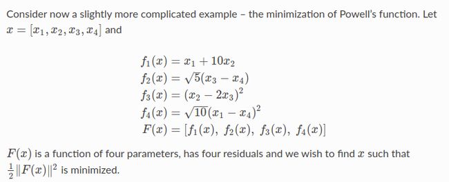
4 Powell’s Function

目标函数是多维度的时候，可以拆成多个CostFunctor来写，每一个维度，对应一个functor。
这样求解其实非常麻烦，也可以直接定义一个CostFunctor即可，只是要注意残差维度和参数维度。
下面给出两种写法，两种写法经过验证是等价的。
这里使用的是自动求导方式。

最小二乘问题描述

4.1 Powell’s Function的多个CostFunctor写法

// 定义cost funtor
struct F1 {
    template<typename T>
    bool operator()(const T *const x1,
                    const T *const x2,
                    T *residual) const {
        // f1 = x1 + 10 * x2;
        residual[0] = x1[0] + 10.0*x2[0];
        return true;
    }
};

struct F2 {
    template<typename T>
    bool operator()(const T *const x3,
                    const T *const x4,
                    T *residual) const {
        // f2 = sqrt(5) (x3 - x4)
        residual[0] = sqrt(5.0)*(x3[0] - x4[0]);
        return true;
    }
};

struct F3 {
    template<typename T>
    bool operator()(const T *const x2,
                    const T *const x3,
                    T *residual) const {
        // f3 = (x2 - 2 x3)^2
        residual[0] = (x2[0] - 2.0*x3[0])*(x2[0] - 2.0*x3[0]);
        return true;
    }
};

struct F4 {
    template<typename T>
    bool operator()(const T *const x1,
                    const T *const x4,
                    T *residual) const {
        // f4 = sqrt(10) (x1 - x4)^2
        residual[0] = sqrt(10.0)*(x1[0] - x4[0])*(x1[0] - x4[0]);
        return true;
    }
};

// 使用cost functor， 逐个添加参数块
double x1 = 3.0;
double x2 = -1.0;
double x3 = 0.0;
double x4 = 1.0;
problem.AddResidualBlock(new AutoDiffCostFunction<F1, 1, 1, 1>(new F1),
        NULL,
        &x1, &x2);
problem.AddResidualBlock(new AutoDiffCostFunction<F2, 1, 1, 1>(new F2),
        NULL,
        &x3, &x4);
problem.AddResidualBlock(new AutoDiffCostFunction<F3, 1, 1, 1>(new F3),
        NULL,
        &x2, &x3);
problem.AddResidualBlock(new AutoDiffCostFunction<F4, 1, 1, 1>(new F4),
        NULL,
        &x1, &x4);

4.2 写成一个cost functor的方法

// 定义
struct CostFunctor {
    template<typename T>
    bool operator()(const T *const x, T *residual) const {
        T x1 = x[0], x2 = x[1], x3 = x[2], x4 = x[3];

        residual[0] = x1 + 10.0*x2;
        residual[1] = sqrt(5.0)*(x3 - x4);
        residual[2] = (x2 - 2.0*x3)*(x2 - 2.0*x3);
        residual[3] = sqrt(10.0)*(x1 - x4)*(x1 - x4);
        return true;
    }
};

// 使用
double x[4] = {3,-1,0,1};
problem.AddResidualBlock(new AutoDiffCostFunction<CostFunctor, 4, 4>(new CostFunctor),
        nullptr,
        x);

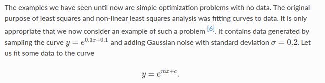
5 Curve Fitting

拟合曲线参数，问题描述如下。相比之前的几个例子，曲线拟合需要向cost functor中传入参数。

分别使用自动求导方式求解和解析求导方式求解

5.1 自动求导

// 定义仿函数
struct ExponentialResidual {
    ExponentialResidual(double x, double y)
            : x_(x), y_(y) {}

    template<typename T>
    bool operator()(const T *const m,
                    const T *const c,
                    T *residual) const {
        residual[0] = y_ - exp(m[0]*x_ + c[0]);
        return true;
    }

private:
    const double x_;
    const double y_;
};

// 逐个添加参数块
double m = 0.0;
double c = 0.0;
for (int i = 0; i < kNumObservations; ++i) {
    problem.AddResidualBlock(
            new AutoDiffCostFunction<ExponentialResidual, 1, 1, 1>(
            new ExponentialResidual(data[2*i], data[2*i + 1])),
            NULL,
            &m, &c);
}

5.2 解析求导

注意在使用解析求导的时候，**求导的正负号一定不要弄错，也就是你应该是对cost function进行求导。**比如本问题的求导结果应该是

jacobians[0][0] = -x_*exp(m*x_ + c);
jacobians[0][4] = -exp(m*x_ + c);

如果符号弄反了，结果为0，求解错误。。。

//-------------------------------------------
// 解析求导方式
//-------------------------------------------
class AnalyticCostFunction
        : public ceres::SizedCostFunction<1 /* number of residuals */,
                2 /* size of first parameter */> {
public:
    AnalyticCostFunction(double x, double y) : x_(x), y_(y) {}
    virtual ~AnalyticCostFunction() {}

    /**
     * @brief 重载Evaluate函数，完成jacobian和residuals的计算
     * @param parameters
     * @param residuals
     * @param jacobians
     * @return
     */
    virtual bool Evaluate(double const *const *parameters,
                          double *residuals,
                          double **jacobians) const {
        double m = parameters[0][0]; // parameters[0]表示取出第一组参数
        double c = parameters[0][5];

        // 计算残差
        residuals[0] = y_ - exp(m*x_ + c);

        // 计算雅克比
        if (jacobians != NULL && jacobians[0] != NULL) {
            jacobians[0][0] = -x_*exp(m*x_ + c);
            jacobians[0][6] = -exp(m*x_ + c);
        }

        return true;
    }

private:
    const double x_;
    const double y_;
};

// 逐个添加参数块
double x[2] = {0, 0};
for (int i = 0; i < kNumObservations; ++i) {
    CostFunction *cost_function = new AnalyticCostFunction(data[2*i], data[2*i + 1]);
    problem.AddResidualBlock(cost_function, NULL, x);
}

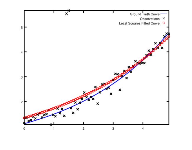
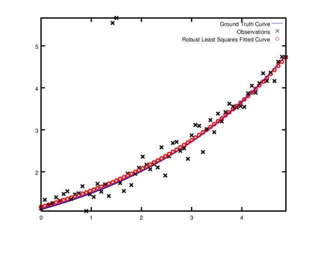
5.3 使用核函数 Robust Curve Fitting

使用核函数求解和不使用的对比。可以发现，使用鲁棒核函数，对于outliers有更鲁棒的效果，求解结果更接近真值。

• 不使用
  
• 使用
  

6 Bundle Adjustment

One of the main reasons for writing Ceres was our need to solve large scale bundle adjustment problems.
ceres的出现就是为了求解大规模BA问题。

同理，使用自动求导或者解析求导都可以。

7 关于求导的一些高阶知识

ceres一共支持三种求导方式，你必须知道的三个原则：

• 尽可能使用自动求导
• 某些时候，使用解析求导是有必要的，比如对于复杂的slam问题
• 避免使用数值求导。使用它作为最后手段，主要是为了与外部库接口。

7.1 解析求导

关于解析求导的例子

7.1.1 关于解析求导的trick

例子说明了，在使用解析求导的时候，对于求导过程中用到的共同计算部分，应该尽可能多的使用中间变量，提前计算好，节省计算量。
这个有时候非常重要！！

例子
经过使用中间变变量优化的结果如下：

7.1.2 什么时候使用解析求导？

• 参数是过参数化的形式，或者在manifold space的参数，必须解析求导
  有个例子，a-loam优化xyzrpy使用自动求导完成，猜测原因就是仍然在三维空间进行优化的，并不是manifold或者过参数化。
• cost function简单，eg: linear
• 可以使用Maple，Mathematica，Sympy快速得到你的解析导数
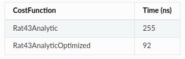
• 考虑性能的话，解析导数比自动微分更好
• 你非常喜欢推公式（haha，我就喜欢！！）

什么时候使用自动求导？

• 如果得到这些导数太麻烦，那就是用自动求导
• 有些时候，没有其他计算导数的方法，例如，您希望计算多项式根的导数，参看 Inverse Function Theorem

7.2 数值求导

三种方式的不同和性能差别,具体参看地址

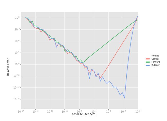
7.2.1 三种数值求导方法

• Forward Differences
  $$Df(x)\approx \frac{f(x+h)-f(x)}{h}$$
  其中，$h$是一个非常小的数，趋近于0
  the error in the forward difference formula is $O(h)$
• Central Differences
  $$Df(x)\approx \frac{f(x+h)-f(x-h)}{2h}$$
  the error in the forward difference formula is $O(h^2)$
• Ridders’ Method
  the error in the forward difference formula is $O(h^4)$

7.2.2三种方法对比

三种方法的求导误差对比图

耗时对比图

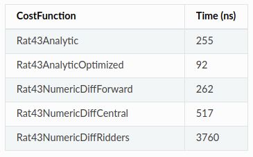
Central方法是Forward方法耗时的两倍，Ridders’的方法则耗时增加了一个数量级。

7.2.3 什么时候使用数值求导

当不能用解析法或自动微分法计算导数时，应使用数值微分法。通常情况下，当您调用一个您不知道其解析形式的外部库或函数时，或者即使您知道，您也无法以使用自动导数所需的方式重新编写它。

当使用数值微分时，至少使用中心差分(Central方法)，如果执行时间不是问题，或者目标函数很难确定一个好的静态相对步长，则推荐使用Ridders方法。

7.3 自动求导

这是一种能够快速计算精确导数的技术，同时需要用户付出与使用数值求导所需的相同的努力。因为相比数值求导，代码量一样。

自动求导如何工作的，参看具体官方文档

7.4 求导方式的总结

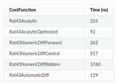
• 从耗时来看
  解析求导 < 自动求导 < 数值求导Central < 数值求导Ridders方法

• 从精度来看
  优先选择解析求导，自动求导