方向梯度直方图HOG
文章目录
-
- 1.关于HOG
- 2.计算x,y方向的梯度 G X G_X GX和 G y G_y Gy
- 3.计算HOG
- 4.skimage计算HOG
- 参考资料
欢迎访问个人网络日志知行空间
1.关于HOG
HOG是2005年发表的论文Histograms of Oriented Gradients for Human Detection中提出的,方向梯度直方图Histograms of Oriented Gradients用于早期的行人检测方法,文章至今引用已超过41500次,是一种非常经典的提取图像特征的方法。要想计算HOG需要先计算图像的梯度。
2.计算x,y方向的梯度 G X G_X GX和 G y G_y Gy
图像可以看成是离散二元函数 f ( x , y ) f(x,y) f(x,y),图像梯度就是这个二元离散函数的偏导。
离散二元函数的偏导数可以使用有限差分来近似计算,图像偏导可写成如下形式:
∂ f ( x , y ) ∂ x = f ( x + 1 , y ) − f ( x , y ) ∂ f ( x , y ) ∂ y = f ( x , y + 1 ) − f ( x , y ) \begin{matrix} \frac{\partial f(x,y)}{\partial x} = f(x + 1, y) - f(x, y) \\ \frac{\partial f(x,y)}{\partial y} = f(x, y + 1) - f(x, y) \end{matrix} ∂x∂f(x,y)=f(x+1,y)−f(x,y)∂y∂f(x,y)=f(x,y+1)−f(x,y)
上面是前向差分求梯度,还可以使用后向差分,
∂ f ( x , y ) ∂ x = f ( x , y ) − f ( x − 1 , y ) ∂ f ( x , y ) ∂ y = f ( x , y ) − f ( x , y − 1 ) \begin{matrix} \frac{\partial f(x,y)}{\partial x} = f(x, y) - f(x-1, y) \\ \frac{\partial f(x,y)}{\partial y} = f(x, y) - f(x, y-1) \end{matrix} ∂x∂f(x,y)=f(x,y)−f(x−1,y)∂y∂f(x,y)=f(x,y)−f(x,y−1)
除了前向差分/后向差分外,还可以使用中心差分:
∂ f ( x , y ) ∂ x = f ( x + 1 , y ) − f ( x − 1 , y ) 2 ∂ f ( x , y ) ∂ y = f ( x , y + 1 ) − f ( x , y − 1 ) 2 \begin{matrix} \frac{\partial f(x,y)}{\partial x} = \frac{f(x+1, y) - f(x-1, y)}{2} \\ \frac{\partial f(x,y)}{\partial y} = \frac{f(x, y+1) - f(x, y-1)}{2} \end{matrix} ∂x∂f(x,y)=2f(x+1,y)−f(x−1,y)∂y∂f(x,y)=2f(x,y+1)−f(x,y−1)
可以使用OpenCV种的Sobel函数来求图像的梯度:
grad_x = cv2.Sobel(image, ddepth, 1, 0, ksize=1, borderType=cv2.BORDER_DEFAULT)
上面代码dx=1,dy=0表示求图像x方向的一阶导数,ksize=1表示使用的是1x3的卷积核,如下:
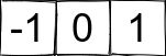
grad_y = cv2.Sobel(image, ddepth, 0, 1, ksize=1, borderType=cv2.BORDER_DEFAULT)
上面代码dx=0,dy=1表示求图像y方向的一阶导数,ksize=1表示使用的是3x1的卷积核,如下:

borderType表示的是对图像边沿的处理方式,OpenCV中给出的图像边沿处理方式有:
| Enumerator | |
|---|---|
| BORDER_CONSTANT
Python: cv.BORDER_CONSTANT
|
|
| BORDER_REPLICATE
Python: cv.BORDER_REPLICATE
|
|
| BORDER_REFLECT
Python: cv.BORDER_REFLECT
|
|
| BORDER_WRAP
Python: cv.BORDER_WRAP
|
|
| BORDER_REFLECT_101
Python: cv.BORDER_REFLECT_101
|
|
| BORDER_TRANSPARENT
Python: cv.BORDER_TRANSPARENT
|
|
| BORDER_REFLECT101
Python: cv.BORDER_REFLECT101
|
same as BORDER_REFLECT_101 |
| BORDER_DEFAULT
Python: cv.BORDER_DEFAULT
|
same as BORDER_REFLECT_101 |
| BORDER_ISOLATED
Python: cv.BORDER_ISOLATED
|
do not look outside of ROI |
如下图,是一幅图像x,y方向梯度求解的过程
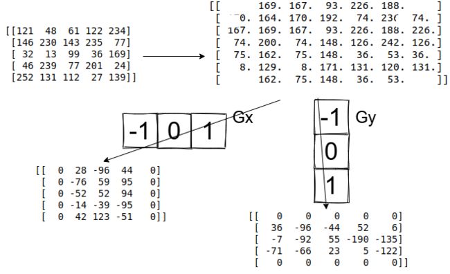
求得 G x G_x Gx和 G y G_y Gy后,再求根据如下公式求梯度的幅值和角度:
G = G x 2 + G y 2 θ = a r t a n G y G x \begin{matrix} G=\sqrt[]{G_x^2+G_y^2} \\ \theta =artan\frac{G_y}{G_x} \end{matrix} G=Gx2+Gy2θ=artanGxGy
使用OpenCV中提供的函数可以很方便的求得上面的两个值:
mag, angle = cv2.cartToPolar(np.float64(grad_x), np.float64(grad_y), angleInDegrees=True)
到这里就计算得到了图像的梯度,下面开始介绍方向梯度直方图。
3.计算HOG
得到一幅图像的梯度后,接下来将图像分成cwxch大小的cell,cw和ch通常取为8x8,cw和ch的选择要结合自己的图像数据,HOG最早应用在行人识别上,图像大小为64×128,因此8x8的cell足以用来表示人体的特征,如人脸等。
对于图像的每个8x8的cell,取对应的梯度幅值和角度,如下图:

将梯度角度分成bins份来绘制8x8 cell中的梯度直方图,如分成9份,对应的角度分别为0,20,40,60,...160。上图中间的小图中,箭头表示梯度方向,箭头长度表示梯度幅值的大小。右边的图中梯度角度的范围为[0, 180],只表示是水平边沿还是垂直边沿,并不判断上下左右,被称为"无符号梯度"。
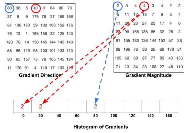
如上图表示一个cell梯度直方图的生成过程,蓝色位置,角度为80,幅值为2,加到对应直方图向量上,红色位置,角度为10,幅值为4,分到0处的梯度幅值 20 − 10 20 × 4 = 2 \frac{20-10}{20}\times 4=2 2020−10×4=2,分到20处的梯度幅值 10 − 0 20 × 4 = 2 \frac{10-0}{20}\times 4=2 2010−0×4=2。同样,对于其他位置的计算也类似。特别的,当角度为165幅度为85时,将幅值对应到0度和160度上算直方图,分到0处的梯度幅值 165 − 160 20 × 85 = 21.25 \frac{165-160}{20}\times 85=21.25 20165−160×85=21.25,分到160处的梯度幅值 20 − ( 165 − 160 ) 20 × 85 = 63.75 \frac{20-(165-160)}{20}\times 85=63.75 2020−(165−160)×85=63.75。最后可以求得一个cell的梯度直方图如下:

根据前面介绍的梯度计算过程,可知梯度幅度受光照影响大,当灰度值变大时,梯度值也会跟着变大,为了减小光照的影响,可以对梯度直方图做归一化。
对彩色像素 [ 128 , 64 , 32 ] [128, 64, 32] [128,64,32],使用L2范数的归一化过程为:
0.87 = 128 12 8 2 + 6 4 2 + 3 2 2 0.43 = 64 12 8 2 + 6 4 2 + 3 2 2 0.22 = 32 12 8 2 + 6 4 2 + 3 2 2 \begin{matrix} 0.87 = \frac{128}{\sqrt{128^2 + 64^2 + 32^2}} \\ 0.43 = \frac{64}{\sqrt{128^2 + 64^2 + 32^2}} \\ 0.22 = \frac{32}{\sqrt{128^2 + 64^2 + 32^2}} \end{matrix} 0.87=1282+642+3221280.43=1282+642+322640.22=1282+642+32232
上面,当向量变成 [ 256 , 128 , 64 ] [256, 128, 64] [256,128,64]后依然有相同的归一化后的值。
HOG的计算中,会将2x2个前面介绍的8x8 cell组合到一起成block,将每个cell的直方图向量拼接到一起,作为这个block的特征向量。前面介绍的每个cell的直方图包含9个bin,组合后每个block包含36个bin,对这个36个元素的向量使用L2范数归一化得到每个block的特征向量。

4.skimage计算HOG
代码来自skimage手册
import matplotlib.pyplot as plt
from skimage.feature import hog
from skimage import data, exposure
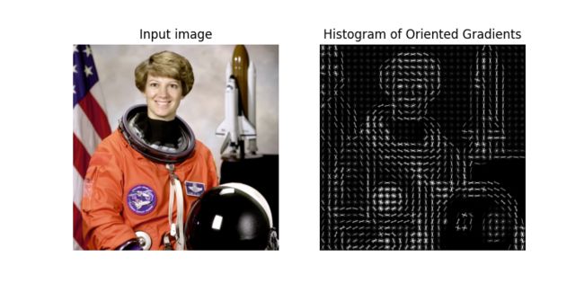
image = data.astronaut()
fd, hog_image = hog(image, orientations=8, pixels_per_cell=(16, 16),
cells_per_block=(1, 1), visualize=True, channel_axis=-1)
fig, (ax1, ax2) = plt.subplots(1, 2, figsize=(8, 4), sharex=True, sharey=True)
ax1.axis('off')
ax1.imshow(image, cmap=plt.cm.gray)
ax1.set_title('Input image')
# Rescale histogram for better display
hog_image_rescaled = exposure.rescale_intensity(hog_image, in_range=(0, 10))
ax2.axis('off')
ax2.imshow(hog_image_rescaled, cmap=plt.cm.gray)
ax2.set_title('Histogram of Oriented Gradients')
plt.show()
参考资料
- 1.https://learnopencv.com/histogram-of-oriented-gradients/
- 2.https://github.com/ahmedfgad/HOGNumPy/blob/master/HOG.py
- 3.https://scikit-image.org/docs/stable/auto_examples/features_detection/plot_hog.html