Deep Learning with Python 系列笔记(三):计算机视觉
计算机视觉的深度学习
我们将深入探讨卷积的原理以及为什么它们在计算机视觉任务中如此成功。但首先,让我们来看看一个非常简单的“convnet”示例,我们将使用我们的convnet来对MNIST数字进行分类。
下面的6行代码展示了基本的convnet是什么样子的。它是一系列 Conv 2d和MaxPooling2D层。我们马上就会看到他们具体做了什么。重要的是,一个convnet作为形状的输入张量(image_height, image_width, image_channel)(不包括批处理维度)。
我们的convnet处理大小的输入(28,28,1),这是MNIST图像的格式。我们通过将参数input_shape=(28,28,1)传递到我们的第一层。
实例化一个小的卷积层
from keras import layers
from keras import models
model = models.Sequential()
model.add(layers.Conv2D(32, (3, 3), activation='relu', input_shape=(28, 28, 1)))
model.add(layers.MaxPooling2D((2, 2)))
model.add(layers.Conv2D(64, (3, 3), activation='relu'))
model.add(layers.MaxPooling2D((2, 2)))
model.add(layers.Conv2D(64, (3, 3), activation='relu'))
展示网络层:
>>> model.summary()
________________________________________________________________
Layer (type) Output Shape Param #
================================================================
conv2d_1 (Conv2D) (None, 26, 26, 32) 320
________________________________________________________________
maxpooling2d_1 (MaxPooling2D) (None, 13, 13, 32) 0
________________________________________________________________
conv2d_2 (Conv2D) (None, 11, 11, 64) 18496
________________________________________________________________
maxpooling2d_2 (MaxPooling2D) (None, 5, 5, 64) 0
________________________________________________________________
conv2d_3 (Conv2D) (None, 3, 3, 64) 36928
================================================================
Total params: 55,744
Trainable params: 55,744
Non-trainable params: 0
你可以在上面看到,每个Conv2D和MaxPooling2D层的输出都是一个三维的形状张量(高度、宽度、通道)。随着网络的深入,宽度和高度都会缩小。通道的数量由传递给Conv2D层的第一个参数控制(例如32或64)。
一步是将我们的最后一个输出张量(形状(3,3,64))输入到一个与你已经熟悉的、紧密相连的分类器网络中:一堆全连接层。这些分类器处理向量,它们是1D,而我们现在的输出是一个3D张量。首先,我们要把3D输出压平到1D,然后在上面再加一些稠密的层。
model.add(layers.Flatten())
model.add(layers.Dense(64, activation='relu'))
model.add(layers.Dense(10, activation='softmax'))

>>> model.summary()
Layer (type) Output Shape Param #
================================================================
conv2d_1 (Conv2D) (None, 26, 26, 32) 320
________________________________________________________________
maxpooling2d_1 (MaxPooling2D) (None, 13, 13, 32) 0
________________________________________________________________
conv2d_2 (Conv2D) (None, 11, 11, 64) 18496
________________________________________________________________
maxpooling2d_2 (MaxPooling2D) (None, 5, 5, 64) 0
________________________________________________________________
conv2d_3 (Conv2D) (None, 3, 3, 64) 36928
________________________________________________________________
flatten_1 (Flatten) (None, 576) 0
________________________________________________________________
dense_1 (Dense) (None, 64) 36928
________________________________________________________________
dense_2 (Dense) (None, 10) 650
================================================================
Total params: 93,322
Trainable params: 93,322
Non-trainable params: 0
正如你所看到的,我们的(3,3,64)输出被压平成形状的矢量(576,),然后输入全连接层。
from keras.datasets import mnist
from keras.utils import to_categorical
(train_images, train_labels), (test_images, test_labels) = mnist.load_data()
train_images = train_images.reshape((60000, 28, 28, 1))
train_images = train_images.astype('float32') / 255
test_images = test_images.reshape((10000, 28, 28, 1))
test_images = test_images.astype('float32') / 255
train_labels = to_categorical(train_labels)
test_labels = to_categorical(test_labels)
model.compile(optimizer='rmsprop',
loss='categorical_crossentropy',
metrics=['accuracy'])
model.fit(train_images, train_labels, epochs=5, batch_size=64)

>>> test_loss, test_acc = model.evaluate(test_images, test_labels)
>>> test_acc
>0.99080000000000001
卷积操作
经过卷积操作后提取的特征如下:

卷积操作有两个有趣的特性:
- 卷积操作学习的模式是平移不变的,也就是说,在学习了图片右下角的某个模式后,一个convnet可以在任何地方识别它,例如在左上角。对于全连接网络,如果图片特征出现在一个新的位置,那么它就必须重新学习这个模式。这使得在处理图像时,convnets的数据效率非常高(因为visual world基本上是平移不变的):它们需要较少的训练样本来学习具有泛化能力的表示。
- 它们可以学习模式的空间层次结构。第一个卷积层将学习小的局部模式,例如边缘,但是第二个卷积层将学习由第一个层的特征构成的更大的模式。等等。这使得convnets能够有效地学习越来越复杂和抽象的视觉概念(因为视觉世界从根本上是空间层次)。

卷积操作超过3D张量,称为“feature maps”,有两个空间轴(“高度”和“宽度”)以及一个“深度”轴(也称为“通道”轴)。对于RGB图像,“深度”轴的尺寸为3,因为图像有3个颜色通道,红色、绿色和蓝色。对于黑白图像,就像我们的MNIST数字一样,深度只有1(灰度)。卷积操作从它的输入特性映射中提取补丁,并对所有这些补丁应用相同的转换,生成一个输出特性映射。这个输出特性图仍然是一个3D张量:它仍然有一个宽度和一个高度。它的深度可以是任意的,因为输出深度是层的参数,而深度轴的不同通道不再代表特定的颜色,比如RGB输入,它们代表的是我们所说的filters。Filters 对输入数据的特定方面进行编码:例如,在高级别上,单个 filter 可以对“在输入中出现的人脸”进行编码。
在我们的MNIST示例中,第一个卷积层采用大小(28、28、1)的feature map,并输出一个(26,26,32)大小的feature map,即它在其输入上计算32个“filters”。这32个输出通道中的每一个都包含一个26x26的值网格,这是一个 filter 对输入的“响应映射”,指示在输入的不同位置的 filer 模式的响应。这就是术语“feature map”的真正含义:深度轴的每个维度都是一个特性(或 filer ),而2D张量输出[:,n]是这个过滤器对输入的响应的二维空间“映射”。

卷积层由两个关键参数决定:
- 从输入中提取的补丁的大小(通常为3x3或5x5)。在我们的例子中,它总是3x3,这是一个很常见的选择。
- 输出特征图的深度,即由卷积计算的 filers 数。在我们的示例中,我们以32的深度开始,以64的深度结束。
在Keras Conv2D层中,这些参数是传递给层的第一个参数:Conv2D(output_depth, (window_height, window_width))。
通过“滑动”这些大小为3x3或5x5的窗口,通过3D输入feature map,在每个可能的位置停止,并提取周围特性的3D补丁(形状(window_height, window_width, input_depth))。然后,每个这样的3D贴片被转换(通过一个具有相同学习权矩阵的张量乘积,称为“卷积核”)到一个一维的形状向量(output_depth,)。然后将所有这些向量空间重新组合成一个形状(高度、宽度、output_depth)的3D输出图。输出特性映射中的每个空间位置都对应于输入特性映射中的相同位置(例如,输出的右下角包含输入的右下角的信息)。例如,在3x3窗口中,矢量输出[i, j,:]来自3D补丁输入[i-1:i+1, j-1:j+1,:]。

注意,输出的宽度和高度可能与输入的宽度和高度不同。他们可能因两个原因而不同:
- 边界效应,可以通过填充输入特征图来抵消
- “strides”的使用
理解边界效应和填充
考虑一个5x5的feature map(总共25块)。只有9个不同的瓦片,你可以把它放在一个3x3的窗口中,形成一个3x3的网格。因此,输出feature map将是3x3:它会缩小一点,在这个例子中,每一个维度旁边正好有两个方块。您可以在上面的示例中看到这种“边界效应”:我们从28x28输入开始,在第一个卷积层之后,它变成了26x26。

如果您想要获得与输入相同的空间维度的输出特性图,则可以使用 Padding:

在Conv2D层中,填充可以通过padding参数进行配置,该参数采用两个值:“valid”,即没有填充(只使用“valid”窗口位置)和“same”,这意味着“以相同宽度和高度的输出作为输入”,填充参数默认为“valid”。
理解卷积的Strides
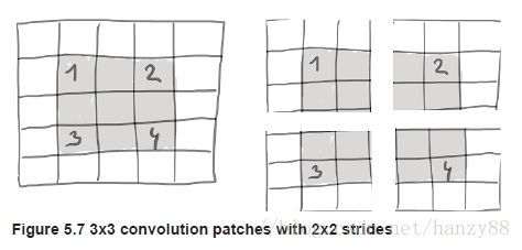
使用stride 2意味着feature map的宽度和高度被一个因子2(除了边界效应所引起的任何变化)所降低。在实践中很少使用带条纹的卷积,尽管它们在某些类型的模型中很有用,但是熟悉这个概念通常很好。
The max pooling operation
在我们的convnet示例中,您可能已经注意到,每个MaxPooling2D层之后,feature map的大小都会减半。例如,在第一个MaxPooling2D层之前,feature map是26x26,但最大池操作将其分为13x13。这就是max pooling的作用:大幅降低样本特征映射,就像跨越的卷积。
a convnet without pooling layers
model_no_max_pool = models.Sequential()
model_no_max_pool.add(layers.Conv2D(32, (3, 3), activation='relu', input_shape=(28, 28, 1)))
model_no_max_pool.add(layers.Conv2D(64, (3, 3), activation='relu'))
model_no_max_pool.add(layers.Conv2D(64, (3, 3), activation='relu'))

>>> model_no_max_pool.summary()
Layer (type) Output Shape Param #
================================================================
conv2d_4 (Conv2D) (None, 26, 26, 32) 320
________________________________________________________________
conv2d_5 (Conv2D) (None, 24, 24, 64) 18496
________________________________________________________________
conv2d_6 (Conv2D) (None, 22, 22, 64) 36928
================================================================
Total params: 55,744
Trainable params: 55,744
Non-trainable params: 0
这一步有什么问题,主要有两方面:
- 它不利于学习特征的空间层次结构。第三层的3x3窗口只包含来自初始输入的7x7窗口的信息。我们的convnet所学习的高级模式在初始输入方面仍然非常小,这可能还不足以学习对数字进行分类(仅通过7x7像素的窗口来识别一个数字)。我们需要从上一个卷积层的特征来包含关于输入全部的信息。
- 最终的feature map有222264 = 31000总系数。这是巨大的。如果我们把它压平,在上面粘上512大小的全连接层,那层就会有1580万个参数。对于这样一个小模型来说,这太大了,会导致过度拟合。
简而言之,使用downsampling的原因仅仅是为了减少特征映射系数的处理次数,以及通过连续的卷积层观察越来越大的窗口来诱导空间过滤层次结构(就其所覆盖的原始输入的分数而言)。
深度学习与小数据的问题
你有时会听到,只有当大量数据可用时,深度学习才会起作用。这在一定程度上是一个有效的观点:深度学习的一个基本特征是,它能够在自己的训练数据中找到有趣的特性,而不需要人工提取的特征工程,只有当大量的训练实例可用时才能实现。对于输入样本非常高维的问题,比如图像,尤其如此。
然而,对于初学者来说,“大量”的样本是相对于你想要训练的网络的大小和深度而言的。仅仅用几十个样本就可以训练一个Convnets网络来解决一个复杂的问题是不可能的,但是如果这个模型是小的,并且有良好的正则化,并且任务简单,那么几百个可能就足够了。
但更重要的是,深度学习模型本质上是高度可重用的。比如,你可以在一个大规模数据集上接受一个图像分类或语音到文本的模型,然后在一个非常不同的问题上重用它,只需要做一些细微的改变。具体地说,在计算机视觉的情况下,许多预先训练过的模型(通常是在ImageNet数据集上进行训练)现在可以公开下载,并且可以通过非常小的数据来引导强大的视觉模型。
Copying images to train,validation and test directories
import os, shutil
# The path to the directory where the original
# dataset was uncompressed
original_dataset_dir = '/Users/Downloads/kaggle_original_data'

# The directory where we will
# store our smaller dataset
base_dir = '/Users/Downloads/cats_and_dogs_small'
os.mkdir(base_dir)

# Directories for our training,
# validation and test splits
train_dir = os.path.join(base_dir, 'train')
os.mkdir(train_dir)
validation_dir = os.path.join(base_dir, 'validation')
os.mkdir(validation_dir)
test_dir = os.path.join(base_dir, 'test')
os.mkdir(test_dir)

# Directory with our training cat pictures
train_cats_dir = os.path.join(train_dir, 'cats')
os.mkdir(train_cats_dir)

# Directory with our training dog pictures
train_dogs_dir = os.path.join(train_dir, 'dogs')
os.mkdir(train_dogs_dir)

# Directory with our validation cat pictures
validation_cats_dir = os.path.join(validation_dir, 'cats')
os.mkdir(validation_cats_dir)

# Directory with our validation dog pictures
validation_dogs_dir = os.path.join(validation_dir, 'dogs')
os.mkdir(validation_dogs_dir)

# Directory with our test cat pictures
test_cats_dir = os.path.join(test_dir, 'cats')
os.mkdir(test_cats_dir)

# Directory with our test dog pictures
test_dogs_dir = os.path.join(test_dir,'dogs')
os.mkdir(test_dogs_dir)

# Copy first 1000 cat images to train_cats_dir
fnames = ['cat.{}.jpg'.format(i) for i in range(1000)]
for fname in fnames:
	src = os.path.join(original_dataset_dir, fname)
	dst = os.path.join(train_cats_dir, fname)
	shutil.copyfile(src, dst)

# Copy next 500 cat images to validation_cats_dir
fnames = ['cat.{}.jpg'.format(i) for i in range(1000, 1500)]
for fname in fnames:
	src = os.path.join(original_dataset_dir, fname)
	dst = os.path.join(validation_cats_dir,fname)
	shutil.copyfile(src, dst)

# Copy next 500 cat images to test_cats_dir
fnames = ['cat.{}.jpg'.format(i) for i in range(1500, 2000)]
for fname in fnames:
	src = os.path.join(original_dataset_dir, fname)
	dst = os.path.join(test_cats_dir, fname)
	shutil.copyfile(src, dst)

# Copy first 1000 dog images to train_dogs_dir
fnames = ['dog.{}.jpg'.format(i) for i in range(1000)]
for fname in fnames:
	src = os.path.join(original_dataset_dir, fname)
	dst = os.path.join(train_dogs_dir, fname)
	shutil.copyfile(src, dst)

# Copy next 500 dog images to validation_dogs_dir
fnames = ['dog.{}.jpg'.format(i) for i in range(1000, 1500)]
for fname in fnames:
	src = os.path.join(original_dataset_dir, fname)
	dst = os.path.join(validation_dogs_dir, fname)
	shutil.copyfile(src, dst)

# Copy next 500 dog images to test_dogs_dir
fnames = ['dog.{}.jpg'.format(i) for i in range(1500, 2000)]
for fname in fnames:
	src = os.path.join(original_dataset_dir, fname)
	dst = os.path.join(test_dogs_dir, fname)
	shutil.copyfile(src, dst)
Counting the images
>>> print('total training cat images:', len(os.listdir(train_cats_dir)))
total training cat images: 1000
>>> print('total training dog images:', len(os.listdir(train_dogs_dir)))
total training dog images: 1000
>>> print('total validation cat images:', len(os.listdir(validation_cats_dir)))
total validation cat images: 500
>>> print('total validation dog images:', len(os.listdir(validation_dogs_dir)))
total validation dog images: 500
>>> print('total test cat images:', len(os.listdir(test_cats_dir)))
total test cat images: 500
>>> print('total test dog images:', len(os.listdir(test_dogs_dir)))
total test dog images: 500
搭建网络
注意,feature map的深度在网络中逐渐增加(从32到128),而feature map的大小正在减少(从148x148到7x7)。这是一个在几乎所有的Convnets 中都能看到的模式。
from keras import layers
from keras import models

model = models.Sequential()
model.add(layers.Conv2D(32, (3, 3), activation='relu',
		input_shape=(150, 150, 3)))
model.add(layers.MaxPooling2D((2, 2)))
model.add(layers.Conv2D(64, (3, 3), activation='relu'))
model.add(layers.MaxPooling2D((2, 2)))
model.add(layers.Conv2D(128, (3, 3), activation='relu'))
model.add(layers.MaxPooling2D((2, 2)))
model.add(layers.Conv2D(128, (3, 3), activation='relu'))
model.add(layers.MaxPooling2D((2, 2)))
model.add(layers.Flatten())
model.add(layers.Dense(512, activation='relu'))
model.add(layers.Dense(1, activation='sigmoid'))
让我们来看看特征映射的维度是如何随着每一个连续的层而变化的。
>>> model.summary()
Layer (type) Output Shape Param #
================================================================
conv2d_1 (Conv2D) (None, 148, 148, 32) 896
________________________________________________________________
maxpooling2d_1 (MaxPooling2D) (None, 74, 74, 32) 0
________________________________________________________________
conv2d_2 (Conv2D) (None, 72, 72, 64) 18496
________________________________________________________________
maxpooling2d_2 (MaxPooling2D) (None, 36, 36, 64) 0
________________________________________________________________
conv2d_3 (Conv2D) (None, 34, 34, 128) 73856
________________________________________________________________
maxpooling2d_3 (MaxPooling2D) (None, 17, 17, 128) 0
________________________________________________________________
conv2d_4 (Conv2D) (None, 15, 15, 128) 147584
________________________________________________________________
maxpooling2d_4 (MaxPooling2D) (None, 7, 7, 128) 0
________________________________________________________________
flatten_1 (Flatten) (None, 6272) 0
________________________________________________________________
dense_1 (Dense) (None, 512) 3211776
________________________________________________________________
dense_2 (Dense) (None, 1) 513
================================================================
Total params: 3,453,121
Trainable params: 3,453,121
Non-trainable params: 0
编译网络
from keras import optimizers
model.compile(loss='binary_crossentropy',
	optimizer=optimizers.RMSprop(lr=1e-4),
	metrics=['acc'])
数据处理
正如现在已经知道的,在将数据输入到我们的网络之前,数据应该被格式化为适当的预处理的浮点张量。目前,我们的数据以JPEG文件的形式存在,因此将其放入我们的网络的步骤大致是这样的:
- 读取图片文件。
- 将JPEG内容解码为像素的RBG网格。
- 将它们转换为浮点张量。
- 将像素值(从0到255)重新缩放到[0,1]区间 (如你所知,神经网络更喜欢处理小的输入值)。
Keras与图像处理模块的辅助工具,位于keras.preprocessing.image。特别地,它包含类ImageDataGenerator,它允许快速设置Python生成器,可以自动将磁盘上的图像文件转换为成批的预处理的张量。这就是我们要用到的。
用 ImageDataGenerator 读取图片
from keras.preprocessing.image import ImageDataGenerator

# All images will be rescaled by 1./255
train_datagen = ImageDataGenerator(rescale=1./255)
test_datagen = ImageDataGenerator(rescale=1./255)

train_generator = train_datagen.flow_from_directory(
	# This is the target directory
	train_dir,
	# All images will be resized to 150x150
	target_size=(150, 150),
	batch_size=20,
	# Since we use binary_crossentropy loss, we need binary labels
	class_mode='binary')
	# categorical

validation_generator = test_datagen.flow_from_directory(
	validation_dir,
	target_size=(150, 150),
	batch_size=20,
	class_mode='binary')
让我们来看看其中一个生成器的输出:它生成了150×150的RGB图像(形状(20、150、150、3))和二分类标签(形状(20,))。20是每批样品的数量(batch_size)。请注意,生成器无限地生成这些批次:它只是对目标文件夹中的图像无休止地循环。出于这个原因,我们需要在某个时刻打破迭代循环。
Displaying the shapes of a batch of data and labels
>>> for data_batch, labels_batch in train_generator:
>>>    print('data batch shape:', data_batch.shape)
>>>    print('labels batch shape:', labels_batch.shape)
>>>    break
data batch shape: (20, 150, 150, 3)
labels batch shape: (20,)
让我们使用生成器将模型与数据相匹配。我们使用的是fit_generator方法,它相当于我们的数据生成器。它希望作为第一个参数,一个Python生成器能够像我们一样,无限期地产生大量的输入和目标。由于数据是不断生成的,因此生成器需要知道从生成器中抽取多少个样本,然后才宣告一个时代结束。这是steps_per_epoch参数的角色:在从生成器中提取steps_per_epoch批次之后,即在运行steps_per_epoch梯度下降步骤之后,拟合过程将进入下一个阶段。在我们的情况下,批次是20个样品,所以要100个批次,直到我们看到我们的2000个样品的目标。
当使用fit_generator时,您可能会传递validation_data参数,这与fit方法非常相似。重要的是,这个参数可以是一个数据生成器本身,但是它也可以是一组Numpy数组。如果您将生成器作为validation_data传递,那么这个生成器将会不断地生成批次的验证数据,因此您还应该指定validation_steps参数,该参数告诉流程从验证生成器中抽取多少批次进行评估。
history = model.fit_generator(
	train_generator,
	steps_per_epoch=100,
	epochs=30,
	validation_data=validation_generator,
	validation_steps=50)
训练后总是保存模型是很好的习惯。
model.save('cats_and_dogs_small_1.h5')
在训练过程中,让我们在训练和验证数据上画出模型的损失和准确性。
import matplotlib.pyplot as plt

acc = history.history['acc']
val_acc = history.history['val_acc']
loss = history.history['loss']
val_loss = history.history['val_loss']
epochs = range(1, len(acc) + 1)
plt.plot(epochs, acc, 'bo', label='Training acc')
plt.plot(epochs, val_acc, 'b', label='Validation acc')
plt.title('Training and validation accuracy')
plt.legend()
plt.figure()
plt.plot(epochs, loss, 'bo', label='Training loss')
plt.plot(epochs, val_loss, 'b', label='Validation loss')
plt.title('Training and validation loss')
plt.legend()
plt.show()


因为我们只有相对较少的培训样本(2000),解决过拟合将是首选。你已经了解了一些可以帮助减轻过拟合的技术,例如Drop out和weight decay(L2正则化)。我们现在将介绍一种新的,具体到计算机视觉,并且在处理深度学习模型的图像时几乎普遍使用:数据增强。
数据增强
过度拟合是由于样本太少,无法学习,使我们无法训练一个能够推广到新数据的模型。数据增强的方法是从现有的训练样本中生成更多的训练数据,通过一些随机的转换来“增加”样本,这些转换产生可信的图像。我们的目标是在训练的时候,我们的模型永远不会看到完全相同的画面。这有助于模型更深入地了解数据的各个方面,并更好地推广。
在Keras中,可以通过在ImageDataGenerator实例读取的图像上配置一些随机转换来实现这一点。
datagen = ImageDataGenerator(
	rotation_range=40,
	width_shift_range=0.2,
	height_shift_range=0.2,
	shear_range=0.2,
	zoom_range=0.2,
	horizontal_flip=True,
	fill_mode='nearest')
这些只是一些可用的选项(更多的,请参见Keras文档)。回顾一下这些参数:
- rotation_range:取值在(0,180),随机旋转图片的范围。
- width_shift and height_shift:取值范围(作为总宽度或高度的一小部分)是在其中任意地垂直或水平地转换图片。
- shear_range:是随机应用剪切变换。
- zoom_range:是在图片中随机放大。
- horizontal_flip: for randomly flipping half of the images horizontally—relevant when there are no assumptions of horizontal asymmetry (e.g. real-world pictures).
- fill_mode: is the strategy used for filling in newly created pixels, which can appear after a rotation or a width/height shift.
# This is module with image preprocessing utilities
from keras.preprocessing import image

fnames = [os.path.join(train_cats_dir, fname) for fname in os.listdir(train_cats_dir)]

# We pick one image to "augment"
img_path = fnames[3]

# Read the image and resize it
img = image.load_img(img_path, target_size=(150, 150))
# Convert it to a Numpy array with shape (150, 150, 3)
x = image.img_to_array(img)

# Reshape it to (1, 150, 150, 3)
x = x.reshape((1,) + x.shape)

# The .flow() command below generates batches of randomly transformed images.
# It will loop indefinitely, so we need to `break` the loop at some point!
i = 0
for batch in datagen.flow(x, batch_size=1):
	plt.figure(i)
	imgplot = plt.imshow(image.array_to_img(batch[0]))
	i += 1
	if i % 4 == 0:
		break

plt.show()

如果我们使用这个数据扩充配置来训练一个新的网络,我们的网络将不会看到两次相同的输入。但是,它所看到的输入仍然是相互关联的,因为它们来自于少数原始图像,我们不能产生新的信息,我们只能重新组合现有的信息。因此,这可能不足以完全消除过度拟合。为了进一步打击过度拟合,我们还将在我们的模型中添加一个Drop out,在全连接的分类器之前:
Defining a new convnet that includes dropout
model = models.Sequential()
model.add(layers.Conv2D(32, (3, 3), activation='relu',
			input_shape=(150, 150, 3)))
model.add(layers.MaxPooling2D((2, 2)))
model.add(layers.Conv2D(64, (3, 3), activation='relu'))
model.add(layers.MaxPooling2D((2, 2)))
model.add(layers.Conv2D(128, (3, 3), activation='relu'))
model.add(layers.MaxPooling2D((2, 2)))
model.add(layers.Conv2D(128, (3, 3), activation='relu'))
model.add(layers.MaxPooling2D((2, 2)))
model.add(layers.Flatten())
model.add(layers.Dropout(0.5))
model.add(layers.Dense(512, activation='relu'))
model.add(layers.Dense(1, activation='sigmoid'))

model.compile(loss='binary_crossentropy',
		optimizer=optimizers.RMSprop(lr=1e-4),
		metrics=['acc'])
Training our convnet using data augmentation generators
train_datagen = ImageDataGenerator(
	rescale=1./255,
	rotation_range=40,
	width_shift_range=0.2,
	height_shift_range=0.2,
	shear_range=0.2,
	zoom_range=0.2,
	horizontal_flip=True,)

# Note that the validation data should not be augmented!
test_datagen = ImageDataGenerator(rescale=1./255)

train_generator = train_datagen.flow_from_directory(
	# This is the target directory
	train_dir,
	# All images will be resized to 150x150
	target_size=(150, 150),
	batch_size=32,
	# Since we use binary_crossentropy loss, we need binary labels
	class_mode='binary')

validation_generator = test_datagen.flow_from_directory(
	validation_dir,
	target_size=(150, 150),
	batch_size=32,
	class_mode='binary')

history = model.fit_generator(
	train_generator,
	steps_per_epoch=100,
	epochs=100,
	validation_data=validation_generator,
	validation_steps=50)
让我们保存我们的模型,我们将在Convnet网络可视化部分使用它。
model.save('cats_and_dogs_small_2.h5')
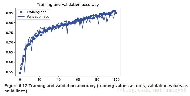
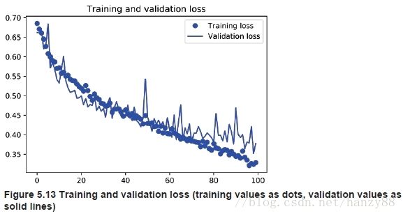
由于数据的增加和Drop out,我们不再过拟合:训练曲线更接近于验证曲线。我们现在能够达到82%的精确度,相对于非正则化模型有15%的相对改进。
使用预先训练的卷积网络
对小图像数据集进行深度学习的一种常见且非常有效的方法是利用预先训练好的网络。一个预先训练的网络只是一个以前在大数据集上训练的保存的网络,通常是大规模的图像分类任务。
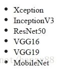
VGG16模型和其他模型一样,都是预先打包的Keras,你可以从 keras.applications 导入它。这里是图像分类模型的列表(都是在ImageNet数据集上预先训练的),作为keras.applications的一部分可用:
实例化模型
from keras.applications import VGG16

conv.base = VGG16(weights = 'imagenet',include_top = False, input_shape=(150,150,3))
函数中传入了三个参数:
**1. weights ?*指定哪个权重检查点来初始化模型。
**2. include_top:**确定是否包括网络中的全连接层,由于原网络中的全连接层会从ImageNet中分出1000类,而在这里我们只做二分类任务,所以不适用。
**3. input_shape:**输入网络的图像张量,如果我们不定义,网络可以处理任何尺寸的输入。
展示VGG16的网络模型:
>>> conv_base.summary()
Layer (type) Output Shape Param #
================================================================
input_1 (InputLayer) (None, 150, 150, 3) 0
________________________________________________________________
block1_conv1 (Convolution2D) (None, 150, 150, 64) 1792
________________________________________________________________
block1_conv2 (Convolution2D) (None, 150, 150, 64) 36928
________________________________________________________________
block1_pool (MaxPooling2D) (None, 75, 75, 64) 0
________________________________________________________________
block2_conv1 (Convolution2D) (None, 75, 75, 128) 73856
________________________________________________________________
block2_conv2 (Convolution2D) (None, 75, 75, 128) 147584
________________________________________________________________
block2_pool (MaxPooling2D) (None, 37, 37, 128) 0
________________________________________________________________
block3_conv1 (Convolution2D) (None, 37, 37, 256) 295168
________________________________________________________________
block3_conv2 (Convolution2D) (None, 37, 37, 256) 590080
________________________________________________________________
block3_conv3 (Convolution2D) (None, 37, 37, 256) 590080
________________________________________________________________
block3_pool (MaxPooling2D) (None, 18, 18, 256) 0
________________________________________________________________
block4_conv1 (Convolution2D) (None, 18, 18, 512) 1180160
________________________________________________________________
block4_conv2 (Convolution2D) (None, 18, 18, 512) 2359808
________________________________________________________________
block4_conv3 (Convolution2D) (None, 18, 18, 512) 2359808
________________________________________________________________
block4_pool (MaxPooling2D) (None, 9, 9, 512) 0
________________________________________________________________
block5_conv1 (Convolution2D) (None, 9, 9, 512) 2359808
________________________________________________________________
block5_conv2 (Convolution2D) (None, 9, 9, 512) 2359808
________________________________________________________________
block5_conv3 (Convolution2D) (None, 9, 9, 512) 2359808
________________________________________________________________
block5_pool (MaxPooling2D) (None, 4, 4, 512) 0
================================================================
Total params: 14,714,688
Trainable params: 14,714,688
Non-trainable params: 0
最后feature map的形状为(4,4,512),这就是我们将在上面连接一个全连接分类器的输入特性。
在这一点上,有两种方法可以进行:
- 在数据集上运行卷积基础,将其输出记录到一个Numpy数组中,然后将这些数据作为输入,作为全连接层分类器的输入。这个解决方案是非常快且方便的,因为它只需要为每个输入图像运行一次卷积基础,而卷积基是目前为止网络中最负责的部分。然而,出于同样的原因,这种技术不允许我们利用数据增强。
- 通过在添加全连接层来扩展模型(conv_base),并在输入数据上运行整个端到端。这允许我们使用数据增强,因为每次输入图像都是通过模型看到的卷积基。然而,出于同样的原因,这种技术要比第一个技术负责得多。
我们将介绍这两种技术。让我们遍历设置第一种方法所需的代码:记录我们数据上的conv_base的输出,并将这些输出作为新模型的输入。
Extracting features using the pre-trained convolutional base
import os
import numpy as np
from keras.preprocessing.image import ImageDataGenerator

base_dir = '/Users/fchollet/Downloads/cats_and_dogs_small'
train_dir = os.path.join(base_dir, 'train')
validation_dir = os.path.join(base_dir, 'validation')
test_dir = os.path.join(base_dir, 'test')

datagen = ImageDataGenerator(rescale=1./255)
batch_size = 20

def extract_features(directory, sample_count):
	features = np.zeros(shape=(sample_count, 4, 4, 512))
	labels = np.zeros(shape=(sample_count))
	generator = datagen.flow_from_directory(
		directory,
		target_size=(150, 150),
		batch_size=batch_size,
		class_mode='binary')
	i = 0

	for inputs_batch, labels_batch in generator:
		features_batch = conv_base.predict(inputs_batch)
		features[i * batch_size : (i + 1) * batch_size] = features_batch
		labels[i * batch_size : (i + 1) * batch_size] = labels_batch
		i += 1
		if i * batch_size >= sample_count:
			# Note that since generators yield data indefinitely in a loop,
			# we must `break` after every image has been seen once.
			break
	return features, labels

train_features, train_labels = extract_features(train_dir, 2000)
validation_features, validation_labels = extract_features(validation_dir, 1000)
test_features, test_labels = extract_features(test_dir, 1000)
提取的特征目前是形状(samples,4,4,512)。我们将会把它们输出给全连接层,所以首先我们必须把它们压平为(samples,8192)。
train_features = np.reshape(train_features, (2000, 4 * 4 * 512))
validation_features = np.reshape(validation_features, (1000, 4 * 4 * 512))
test_features = np.reshape(test_features, (1000, 4 * 4 * 512))
此时,我们要定义一个全连接层,注意使用Drop out来正则化,并在刚才提取的特征上训练数据:
from keras import models
from keras import layers
from keras import optimizers
model = models.Sequential()
model.add(layers.Dense(256, activation='relu', input_dim=4 * 4 * 512))
model.add(layers.Dropout(0.5))
model.add(layers.Dense(1, activation='sigmoid'))
model.compile(optimizer=optimizers.RMSprop(lr=2e-5),
			loss='binary_crossentropy',
			metrics=['acc'])

history = model.fit(train_features, train_labels,
					epochs=30,
					batch_size=20,
					validation_data=(validation_features, validation_labels))
训练是非常快的,因为我们只需要处理两个全连接层,一个epoch 即使在CPU上也只需要不到一秒的时间。
import matplotlib.pyplot as plt

acc = history.history['acc']
val_acc = history.history['val_acc']
loss = history.history['loss']
val_loss = history.history['val_loss']

epochs = range(1, len(acc) + 1)
plt.plot(epochs, acc, 'bo', label='Training acc')
plt.plot(epochs, val_acc, 'b', label='Validation acc')
plt.title('Training and validation accuracy')
plt.legend()

plt.figure()

plt.plot(epochs, loss, 'bo', label='Training loss')
plt.plot(epochs, val_loss, 'b', label='Validation loss')
plt.title('Training and validation loss')
plt.legend()

plt.show()

我们达到了大约90%的验证精度,比我们在上一节中通过从头开始训练的小模型所能达到的效果要好得多。然而,结果也表明,尽管我们Drop out的值相当高,但我们几乎从一开始就过拟合。这是因为该技术不利用数据增强,这对于防止小型图像数据集的过度拟合是至关重要的。
Adding a densely-connected classifier on top of the convolutional base
因为模型的行为就像层一样,你可以将一个模型(比如我们的conv_base)添加到一个序列模型中,就像你添加一个层一样。你可以这样做:
from keras import models
from keras import layers

model = models.Sequential()
model.add(conv_base)
model.add(layers.Flatten())
model.add(layers.Dense(256, activation='relu'))
model.add(layers.Dense(1, activation='sigmoid'))
模型现在是这个样子:
>>> model.summary()
Layer (type) Output Shape Param #
================================================================
vgg16 (Model) (None, 4, 4, 512) 14714688
________________________________________________________________
flatten_1 (Flatten) (None, 8192) 0
________________________________________________________________
dense_1 (Dense) (None, 256) 2097408
________________________________________________________________
dense_2 (Dense) (None, 1) 257
================================================================
Total params: 16,812,353
Trainable params: 16,812,353
Non-trainable params: 0
如你所见,VGG16的卷积基础有14,714,688个参数,非常大。我们在上面添加的分类器有200万个参数。
在我们编译和训练我们的模型之前,要做的一件非常重要的事情是***冻结卷积基***。“Freezing”一层或一套层意味着在训练期间防止他们的weight得到更新。如果我们不这样做,那么之前在卷积基础上学习的表示会在训练过程中被修改。由于顶部的全连接层是随机初始化的,所以非常大的权重更新将通过网络传播,从而会破坏之前卷积学到的内容。
>>> print('This is the number of trainable weights '
		'before freezing the conv base:', len(model.trainable_weights))
This is the number of trainable weights before freezing the conv base: 30
>>> conv_base.trainable = False
>>> print('This is the number of trainable weights '
		'after freezing the conv base:', len(model.trainable_weights))
This is the number of trainable weights after freezing the conv base: 4
有了这个设置,只有我们添加的两个全连接层的权重将被训练。这是一个总共有4个分量的张量:每层2个(主要的权重矩阵和偏置向量)。请注意,为了使这些更改生效,我们必须首先编译模型。如果您在编译后修改了weight trainability,那么应该重新编译模型,否则这些更改将被忽略。
from keras.preprocessing.image import ImageDataGenerator

train_datagen = ImageDataGenerator(
	rescale=1./255,
	rotation_range=40,
	width_shift_range=0.2,
	height_shift_range=0.2,
	shear_range=0.2,
	zoom_range=0.2,
	horizontal_flip=True,
	fill_mode='nearest')

# Note that the validation data should not be augmented!
test_datagen = ImageDataGenerator(rescale=1./255)

train_generator = train_datagen.flow_from_directory(
		# This is the target directory
train_dir,
		# All images will be resized to 150x150
		target_size=(150, 150),
		batch_size=20,
		# Since we use binary_crossentropy loss, we need binary labels
		class_mode='binary')

validation_generator = test_datagen.flow_from_directory(
		validation_dir,
		target_size=(150, 150),
		batch_size=20,
		class_mode='binary')

model.compile(loss='binary_crossentropy',
		optimizer=optimizers.RMSprop(lr=2e-5),
		metrics=['acc'])

history = model.fit_generator(
		train_generator,
		steps_per_epoch=100,
		epochs=30,
		validation_data=validation_generator,
		validation_steps=50)

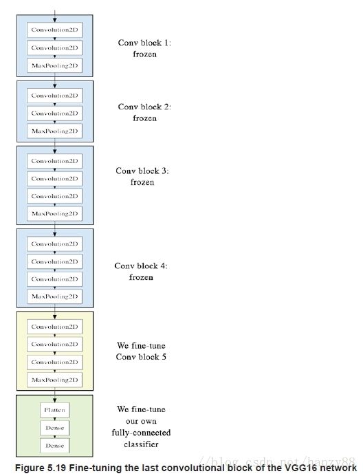
Fine - tuning
另一种广泛使用的用于模型重用的技术是fine-tuning。fine-tuning包括解冻用于特征提取的冻结模型库的几个顶层,并联合培训新添加的模型(在我们的示例中是全连接的分类器)和这些顶层。这被称为“Fine - tuning”,因为它稍微调整了被重用模型的更抽象表示,以便使它们更适合于手头的问题。
我们之前已经说过,为了能够在上面训练一个随机初始化的分类器,需要冻结VGG16的卷积基础。出于同样的原因,一旦上面的分类器已经被训练,它只可能调整卷积基础的顶层。如果分类没有经过训练,那么在训练过程中通过网络传播的错误信号将会太大,而之前被调整的层所得到的表示将被破坏。因此,对网络进行Fine - tuning 的步骤如下:
- 在已经训练好的基础网络上加自定义的网络
- 冻结基础网络
- 训练增加的网络部分
- 解冻基础网络中的一些层
- 一起训练这些解冻层和增加层
在进行特征提取时,我们已经完成了前三个步骤。让我们继续第4步:我们将解冻我们的conv_base,然后冻结它内部的各个层。
>>> conv_base.summary()
Layer (type) Output Shape Param #
================================================================
input_1 (InputLayer) (None, 150, 150, 3) 0
________________________________________________________________
block1_conv1 (Convolution2D) (None, 150, 150, 64) 1792
________________________________________________________________
block1_conv2 (Convolution2D) (None, 150, 150, 64) 36928
________________________________________________________________
block1_pool (MaxPooling2D) (None, 75, 75, 64) 0
________________________________________________________________
block2_conv1 (Convolution2D) (None, 75, 75, 128) 73856
________________________________________________________________
block2_conv2 (Convolution2D) (None, 75, 75, 128) 147584
________________________________________________________________
block2_pool (MaxPooling2D) (None, 37, 37, 128) 0
________________________________________________________________
block3_conv1 (Convolution2D) (None, 37, 37, 256) 295168
________________________________________________________________
block3_conv2 (Convolution2D) (None, 37, 37, 256) 590080
________________________________________________________________
block3_conv3 (Convolution2D) (None, 37, 37, 256) 590080
________________________________________________________________
block3_pool (MaxPooling2D) (None, 18, 18, 256) 0
________________________________________________________________
block4_conv1 (Convolution2D) (None, 18, 18, 512) 1180160
________________________________________________________________
block4_conv2 (Convolution2D) (None, 18, 18, 512) 2359808
________________________________________________________________
block4_conv3 (Convolution2D) (None, 18, 18, 512) 2359808
________________________________________________________________
block4_pool (MaxPooling2D) (None, 9, 9, 512) 0
________________________________________________________________
block5_conv1 (Convolution2D) (None, 9, 9, 512) 2359808
________________________________________________________________
block5_conv2 (Convolution2D) (None, 9, 9, 512) 2359808
________________________________________________________________
block5_conv3 (Convolution2D) (None, 9, 9, 512) 2359808
________________________________________________________________
block5_pool (MaxPooling2D) (None, 4, 4, 512) 0
================================================================
Total params: 14714688
我们将对最后的3个卷积层进行 Fine - tuning,这意味着直到block4_pool应该被冻结,并且层block5_conv1, block5_conv2和block5_conv3应该是可训练的。
为什么不调整更多的层次呢?为什么不微调整个卷积基础?我们可以。然而,我们需要考虑:
- 在卷积基础上,较早的层可以编码更通用的、可重用的特性,而层次较高的则可以编码更专门化的特性。对更专门化的特性进行微调更有用,因为这些特性需要对我们的新问题进行重新规划。
- 我们训练的参数越多,就越有可能被过度拟合。卷积基有15M个参数,所以尝试在我们的小数据集上训练它是有风险的。
因此,在我们的情况下,在卷积基础上只调整前2到3层是一个很好的策略。
conv_base.trainable = True

set_trainable = False
for layer in conv_base.layers:
	if layer.name == 'block5_conv1':
	set_trainable = True
	if set_trainable:
		layer.trainable = True
	else:
		layer.trainable = False
现在我们可以开始微调我们的网络了。我们将使用一个非常低的学习速率来使用RMSprop优化器。使用低学习率的原因是,我们想要限制我们对三层的表示的修改的大小,我们正在进行微调。太大的更新可能会损害这些表示。
model.compile(loss='binary_crossentropy',
		optimizer=optimizers.RMSprop(lr=1e-5),
		metrics=['acc'])

history = model.fit_generator(
	train_generator,
	steps_per_epoch=100,
	epochs=100,
	validation_data=validation_generator,
	validation_steps=50)
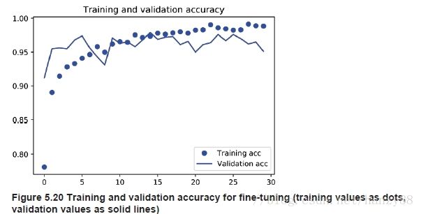
这些曲线看起来有很多Noise。为了使它们更具可读性,我们可以通过用指数移动的平均数来替换每一个损失和精度来使它们平滑。这里是一个平凡的效用函数。
Smoothing our plots:
def smooth_curve(points, factor=0.8):
	smoothed_points = []
	for point in points:
		if smoothed_points:
			previous = smoothed_points[-1]
			smoothed_points.append(previous * factor + point * (1 - factor))
		else:
			smoothed_points.append(point)
	return smoothed_points

plt.plot(epochs,
	smooth_curve(acc), 'bo', label='Smoothed training acc')
plt.plot(epochs,
	smooth_curve(val_acc), 'b', label='Smoothed validation acc')
plt.title('Training and validation accuracy')
plt.legend()
plt.figure()

plt.plot(epochs,
	smooth_curve(loss), 'bo', label='Smoothed training loss')
plt.plot(epochs,
	smooth_curve(val_loss), 'b', label='Smoothed validation loss')
plt.title('Training and validation loss')
plt.legend()

plt.show()

test_generator = test_datagen.flow_from_directory(
	test_dir,
	target_size=(150, 150),
	batch_size=20,
	class_mode='binary')

test_loss, test_acc = model.evaluate_generator(test_generator, steps=50)
print('test acc:', test_acc)
总结
这是你应该从之前的内容学到的:
- Convnets是计算机视觉任务的最好的机器学习模型。即使是在非常小的数据集上,也可以从头开始训练一个,结果很好。
- 在一个小数据集上,过拟合将是主要问题。在处理图像数据时,数据增强是一种有效的方法。
- 通过特征提取,很容易在新的数据集上重用现有的convnet。这是一个非常有价值的技术,用于处理小的图像数据集。
- 作为特征提取的补充,可以使用微调,这将适应一个新问题,其中一些是由现有模型学习的。这进一步推动了性能。