帕金森定律
应用计算机视觉 (Applied Computer Vision)
简介 (Introduction)
Parkinson’s disease is often associated with movement disorder symptoms such as tremors and rigidity. These can have a noticeable effect on the handwriting and sketching (drawing)of a person suffering from early stages of the disease [1]. Micrographia, are abnormally small undulations in a persons handwriting, however, have claimed to be difficult to interpret due to the variability in one’s developed handwriting, language, proficiency and education etc [1]. As such, a study conducted in 2017 aimed to improve the diagnosis through a standardized analysis using spirals and waves. In this series of posts, we will analyze the raw images collected in that study and see if we can create a classifier for a patient having Parkinson’s, and draw some conclusions along the way. The data we will be using is hosted on Kaggle [2] with special thanks to Kevin Mader for sharing the dataset upload.
P arkinson病常与运动障碍症状,如震颤和刚性有关。 这些可以对患有该疾病早期阶段的人的笔迹和草图(绘画)产生显着影响[1]。 显微照相术是人类笔迹中异常小的波动,然而,由于人的笔迹,语言,熟练程度和受教育程度等方面的差异,据称难以解释。 因此,2017年进行的一项研究旨在通过使用螺旋和波浪的标准化分析来改善诊断。 在这一系列文章中,我们将分析该研究收集的原始图像,看看是否可以为患有帕金森氏症的患者创建分类器,并一路得出结论。 我们将使用的数据托管在Kaggle [2]上,特别感谢Kevin Mader分享了数据集上传。
In this part 1, we will be conducting some exploratory data analysis and pre-processing the images to create some features that will hopefully be helpful in classification. I am choosing to NOT use a convolutional neural network (CNN) to simply classify the images as this will be black box — without any metric into the underlying differences between the curves/sketches. Instead, we are not simply performing a task of classifying but trying to use image processing to understand and quantify the differences. In a subsequent post, I will compare with a CNN.
在第1部分中,我们将进行一些探索性数据分析并对图像进行预处理,以创建一些有望对分类有所帮助的功能。 我选择不使用卷积神经网络(CNN)来对图像进行简单分类,因为这将是黑盒-曲线/草图之间的潜在差异没有任何度量标准。 相反,我们不仅仅是执行分类任务,而是尝试使用图像处理来理解和量化差异。 在后续文章中,我将与CNN进行比较。
演示地址
Before we begin, disclaimer that this is not meant to be any kind of medical study or test. Please refer to the original paper for details on the actual experiment, which I was not a part of.Zham P, Kumar DK, Dabnichki P, Poosapadi Arjunan S, Raghav S. Distinguishing Different Stages of Parkinson’s Disease Using Composite Index of Speed and Pen-Pressure of Sketching a Spiral. Front Neurol. 2017;8:435. Published 2017 Sep 6. doi:10.3389/fneur.2017.00435
在我们开始之前,请声明这并不意味着要进行任何医学研究或测试。 请参考原始文件的详细信息,实际的实验,我是不是部分of.Zham P,库马尔DK,Dabnichki P,Poosapadi阿晶南S, 帕金森氏病的使用速度和笔的综合指数拉哈夫S. 区分不同阶段-绘制螺旋线的压力 。 前神经元。 2017; 8:435。 2017年9月6日发布。doi:10.3389 / fneur.2017.00435
探索性数据分析 (Exploratory Data Analysis)
First, let us take a look at the images, perform some basic segmentation and start poking around with some potential features of interest. We will be using pandas throughout to store the images and information. For those of you questioning whether you will read this section here is what we will get into: - Thresholding and cleaning- Thickness quantification through nearest neighbors- Skeletonization- Intersections and edge points
开始步骤,让我们来看看图片,执行一些基本的分割,并开始关注着与一些潜在的利益特征。 我们将在整个过程中使用熊猫来存储图像和信息。 对于那些质疑您是否会阅读本节内容的人,我们将了解以下内容:-阈值化和清洁-通过最近的邻居进行厚度量化-骨骼化-交叉点和边缘点
门槛和清洁 (Thresholding and cleaning)
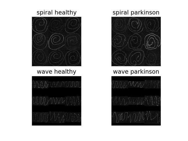
We use a modified read and threshold function, mostly obtained from the original notebook by Kevin Mader on Kaggle [2]. Here, we have the option to perform a resizing when wanting to view the montage style images, like above and below. We first read in and invert the image so the drawings are white on black background, as well as resize if necessary. We also apply a small median filter.
我们使用了修改后的读取和阈值功能,这些功能大部分是由Kevin Mader在Kaggle [2]上的原始笔记本中获得的。 在这里,我们可以选择在想要查看蒙太奇样式图像时执行大小调整,如上方和下方。 我们首先读入图像并将其反转,以使图纸在黑色背景上为白色,并在必要时调整大小。 我们还应用了一个小的中值滤波器。
This project has quite a fair bit of code, I won’t be posting it all here so please see the github link if you want to view the notebook or python script for more details.
这个项目有相当多的代码,我不会在这里发布所有代码,因此如果您想查看笔记本或python脚本以获得更多详细信息,请参见github链接。
from skimage.io import imread
from skimage.util import montage as montage2d
from skimage.filters import threshold_yen as thresh_func
from skimage.filters import median
from skimage.morphology import disk
import numpy as npdef process_imread(in_path, resize=True):
    """read images, invert and scale them"""
    c_img = 1.0-imread(in_path, as_gray=True)
    max_dim = np.max(c_img.shape)
    if not resize:
        return c_img
    if c_img.shape==(256, 256):
        return c_img
    if max_dim>256:
        big_dim = 512
    else:
        big_dim = 256
    """ pad with zeros and center image, sizing to either 256 or 512"""
    out_img = np.zeros((big_dim, big_dim), dtype='float32')
    c_offset = (big_dim-c_img.shape[0])//2
    d_offset = c_img.shape[0]+c_offset
    e_offset = (big_dim-c_img.shape[1])//2
    f_offset = c_img.shape[1]+e_offset
    out_img[c_offset:d_offset, e_offset:f_offset] = c_img[:(d_offset-c_offset), :(f_offset-e_offset)]
    return out_imgdef read_and_thresh(in_path, resize=True):
    c_img = process_imread(in_path, resize=resize)
    c_img = (255*c_img).clip(0, 255).astype('uint8')
    c_img = median(c_img, disk(1))
    c_thresh = thresh_func(c_img)
    return c_img>c_thresh
Lastly, for the read in, we also clean up the images by removing any small objects disconnected from the main sketch.
最后,对于读入,我们还通过移除与主草图断开连接的所有小物体来清理图像。
from skimage.morphology import label as sk_labeldef label_sort(in_img, cutoff=0.01):
    total_cnt = np.sum(in_img>0)
    lab_img = sk_label(in_img)
    new_image = np.zeros_like(lab_img)
    remap_index = []
    for k in np.unique(lab_img[lab_img>0]):
        cnt = np.sum(lab_img==k) # get area of labelled object
        if cnt>total_cnt*cutoff:
            remap_index+=[(k, cnt)]
    sorted_index = sorted(remap_index, key=lambda x: -x[1]) # reverse sort - largest is first
    for new_idx, (old_idx, idx_count) in enumerate(sorted_index, 1): #enumerate starting at id 1
        new_image[lab_img==old_idx] = new_idx
    return new_image
This works by keeping only large enough components that are >1% of activated pixels; defined by cutoff. First label each separate object in the image and sum the areas for each label identified (that isn’t 0). Keep the index if the count is more than 1% of the total. Perform negative sort to have the largest objects with label 1. Replace the old label number with the new ordered id.
通过仅保留大于激活像素的1%的足够大的分量来工作; 由截止定义。 首先标记图像中的每个单独的对象,然后将每个已标识的标签的面积相加(不为0)。 如果计数超过总数的1%,则保留索引。 执行否定排序以使最大的对象带有标签1.将旧标签号替换为新的订购ID。
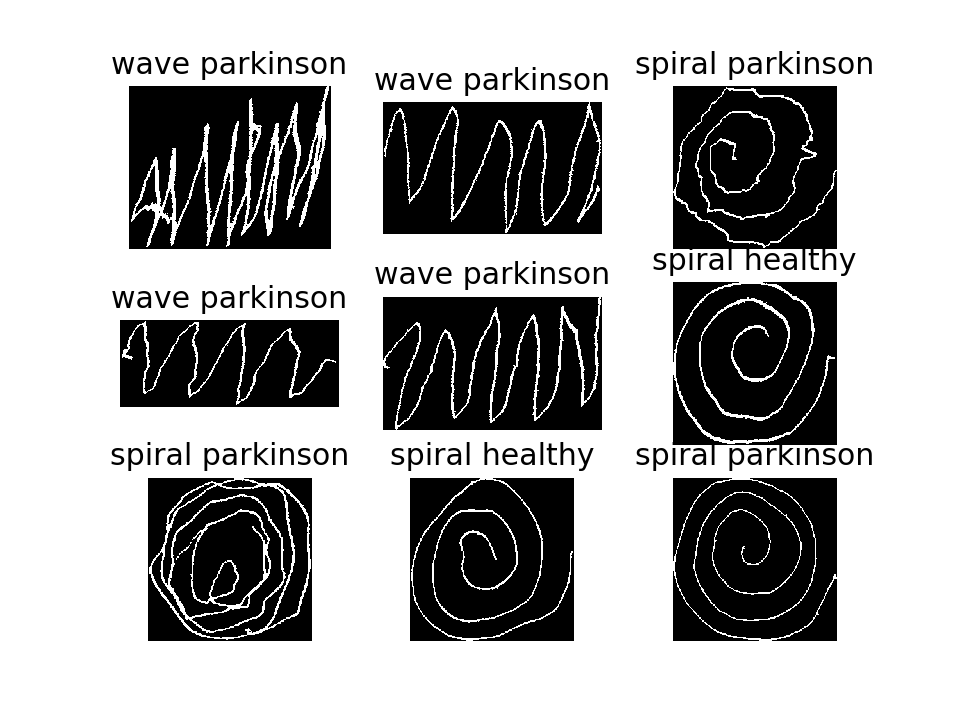
As an initial view of how different the drawings are, we can create a skeleton image and form a new data frame where each row is a single pixel coordinate of non-zero pixels in each image. We can then plot each of these curves on a single graph — after normalizing the positions. We won’t be using this format of the data frame, this is just for visualization.
初步了解图纸的不同之处,我们可以创建一个骨架图像并形成一个新的数据框,其中每一行是每个图像中非零像素的单个像素坐标。 然后,我们可以在对位置进行归一化之后,将这些曲线中的每条曲线绘制在一张图形上。 我们不会使用这种数据框格式,这只是为了可视化。
As we can see there is strong consistency between healthy sketches. This makes sense considering the random motion that Parkinson’s symptoms can cause.
如我们所见,健康草图之间有很强的一致性。 考虑到帕金森氏症可能引起的随机运动,这是有道理的。
厚度定量 (Thickness quantification)
Next, we will try to quantify the thickness. For this, we will be using a distance map to give an approximation of the width of the drawings. The medial axis also returns a distance map, but skeletonize is cleaner as it does some pruning.
ñ分机,我们会尽量量化的厚度。 为此,我们将使用距离图来给出图纸宽度的近似值。 中间轴也返回一个距离图,但是由于进行修剪,骨架化更加清晰。
from skimage.morphology import medial_axis
from skimage.morphology import skeletonizedef stroke_thickness_img(in_img):
    skel, distance = medial_axis(in_img, return_distance=True)
    skeleton = skeletonize(in_img)
    # Distance to the background for pixels of the skeleton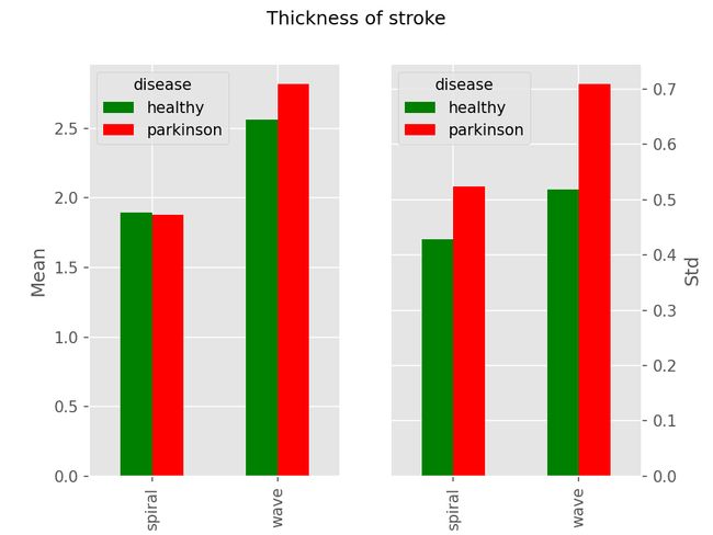
return distance * skeletonPlotting the mean and standard deviation we see some correlation between the drawings. Mostly in the standard deviation which again makes sense considering the random impact, also the fact it is great and not less than healthy also makes sense.
绘制平均值和标准偏差后,我们在图纸之间看到了一些相关性。 大多数情况下,考虑到随机影响,在再次有意义的标准偏差中,也是很大且不少于健康的事实也是有意义的。
交叉点和边缘点 (Intersections and edge-points)
Due to the way that skeletonizing an image works, depending on the ‘smoothness’ of the line, there will be a higher number of end-points for more undulating curves. These are therefore some measure of the random movement compared with a smooth line. In addition, we can calculate the number of intersection points; a perfect curve would have no intersections and only two end-points. These are also useful in other image processing applications such as with road mapping.
d UE到skeletonizing图像作品,这取决于线的“平滑度”的方式,将有更多的起伏曲线的更高数目的端点。 因此,与平滑线相比,这些是随机运动的某种度量。 另外,我们可以计算出相交点的数量; 一条完美的曲线将没有交点,只有两个端点。 这些在其他图像处理应用程序(例如道路地图)中也很有用。
I won’t go into the code too much here as there is a fair bit of cleaning required, however, I will try to explain what I did using some images. First, we calculate a nearest neighbors image of the skeleton of the curve. This gives us values of 2 everywhere, except a value of 1 at edge-points, and a value of 3 at intersections; this is when using a connectivity of 2 (the 8 nearest neighbors). Here is an image of the result, zoomed in.
在这里我不会过多地讨论代码,因为需要进行一些清理工作,但是,我将尝试解释使用某些图像所做的工作。 首先,我们计算曲线骨架的最近邻图像。 这给我们到处都是2的值,除了在边缘点为1的值和在相交处为3的值之外; 这是在使用2(8个最近的邻居)的连通性时。 这是结果的图像,已放大。
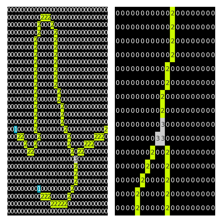
As you can see this works as expected, except we run into some issues if we want to get only one pixel intersection to properly quantify the number of intersections. The image on the right has three pixels with value 3, although this is only one intersection. We can clean this up with the following pseudo algorithm by isolating for these regions as the sum of these intersections is greater than the ‘correct’ intersection. We can sum the nearest neighbors (NN) image and threshold to isolate these. Connectivity 1 has direct neighbors, connected 2 includes diagonals.
如您所见,此方法按预期工作,但如果我们只想获得一个像素交点以正确量化交点数,则会遇到一些问题。 尽管这只是一个交叉点,但右侧的图像具有三个像素,其值为3。 由于这些交点的总和大于“正确”的交点,因此可以通过隔离这些区域使用以下伪算法来清理此问题。 我们可以对最近邻(NN)图像和阈值求和以将其隔离。 连接1具有直接邻居,连接2具有对角线。
- From original NN, sum using connectivity 1 and 2 separately. 从原始NN,分别使用连通性1和2求和。
- Isolate intersections which have value ≥ 8 in connectivity 2. 隔离连接2中值≥8的交叉点。
- Label each edge that is connected to the intersection pixels. 标记连接到相交像素的每个边缘。
- Isolate the intersection pixels which sum between 3 and 5 for the connectivity 1 image. These are the one we don’t want. 隔离连接1图像的相交像素,其总和在3和5之间。 这些是我们不想要的。
- Overwrite incorrect intersection pixels. 覆盖不正确的相交像素。
Here is the result:
结果如下:
As you can see we now have a single pixel with value 3 at the intersection location. We can now simply sum these locations to quantify the number of intersection points. If we draw these on a curve we can see the result, below yellow are intersections and green are edge-points.
如您所见,我们现在在交点位置有一个值为3的单个像素。 现在,我们可以简单地对这些位置求和,以量化相交点的数量。 如果将它们绘制在曲线上,我们可以看到结果,黄色以下是交点,绿色以下是边点。
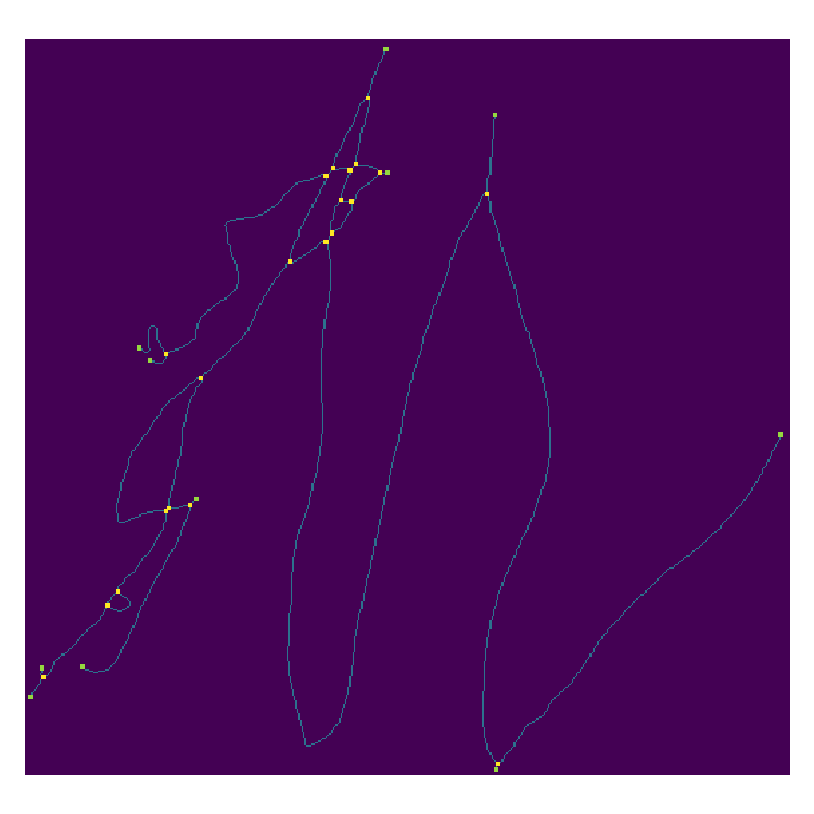
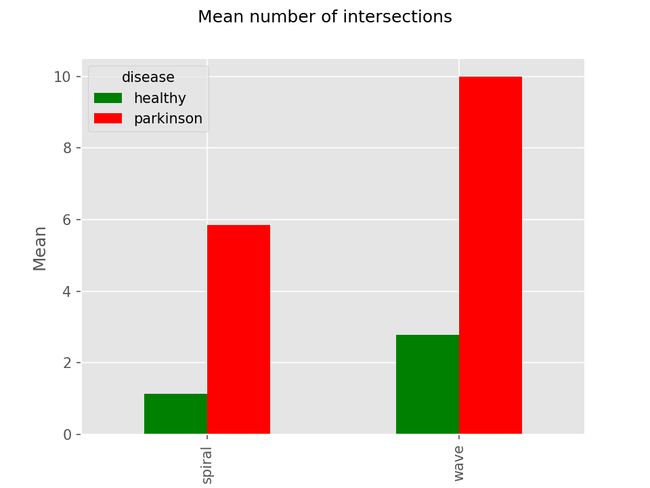
If we plot the number of these for each drawing type we can see the fairly strong correlation:
如果我们为每种图形类型绘制这些图形的数量,我们可以看到相当强的相关性:
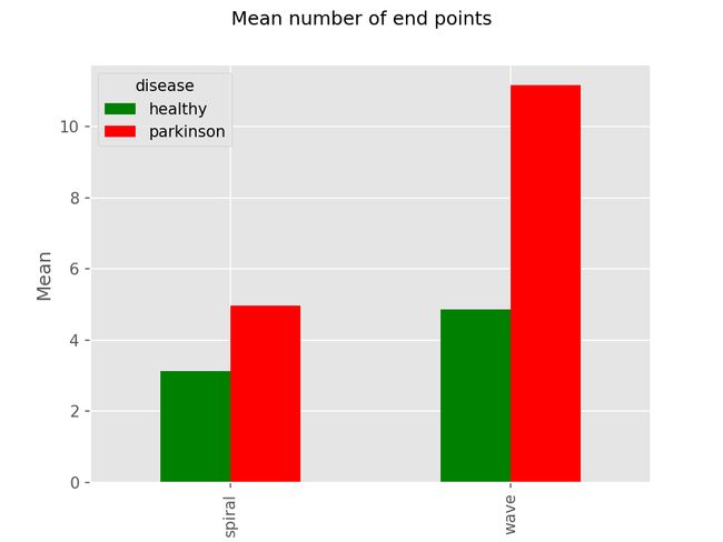
We can also see our initial estimate of a healthy curve having approximately 2 edge-points is also correct. There is a very high number of edge-points for Parkinson’s wave drawings because these are usually quite ‘sharp’ instead of curved smoothly, this creates a high number of edge-points at the tips of these waves.
我们还可以看到对大约2个边缘点的健康曲线的初始估计也是正确的。 帕金森波浪图的边缘点非常多,因为这些边缘点通常非常“锋利”,而不是平滑弯曲,这会在这些波的尖端产生大量边缘点。
Lastly, we can also check the correlation with the overall number of pixels in the skeleton image. This is related to the ‘indirect’ nature of the drawings. This quantification is very simple, we just sum the pixels greater than zero in a skeleton image.
最后,我们还可以检查与骨架图像中像素总数的相关性。 这与附图的“间接”性质有关。 这种量化非常简单,我们只将骨架图像中大于零的像素相加即可。
Not as strong as a relationship but still something.
不如恋爱关系强,但还是有关系。
摘要 (Summary)
So far we have now read in, cleaned and obtained some potentially useful metrics, that help us not only understand the degree of micrographia but also can be used as inputs into a classifier such as Logistic Regression or Random Forest. In part 2 of this series we will perform classification using these metrics and also compare to a more powerful, but black-box, neural network. The advantage of using Random Forest is we will also be able to see which features provide the strongest impact to the model. Based on the above observations, do you have an intuition already about which features may be the most important?
到目前为止,我们现在已经读入,清洗,得到了一些可能有用的指标,可以帮助我们不仅了解写字过小的程度,但也可以作为投入的分类,如Logistic回归或随机森林。 在本系列的第2部分中,我们将使用这些指标进行分类,并与功能更强大的黑匣子神经网络进行比较。 使用随机森林的好处是我们还将能够看到哪些功能对模型的影响最大。 根据以上观察,您是否已经直觉到哪些功能可能是最重要的?
If you felt that any part of this post provided some useful information or just a bit of inspiration please follow me for more.
如果您认为这篇文章的任何部分提供了一些有用的信息或只是一些启发,请关注我以获取更多信息。
You can find the source code on my github. This project is currently still under construction.
您可以在我的github上找到源代码。 该项目目前仍在建设中。
Link to my other posts:
链接到我的其他帖子:
Computer Vision and the Ultimate Pong AI — Using Python and OpenCV to play Pong online
计算机视觉和终极Pong AI —使用Python和OpenCV在线玩Pong
Minecraft Mapper — Computer Vision and OCR to grab positions from screenshots and plot
Minecraft Mapper-计算机视觉和OCR可以从屏幕截图和绘图中获取位置
奖金 (Bonus)
Not used here, but for fun, we can also create a graph for the representation of each image since we have nodes and edges, where the nodes are the intersections or edge-points and the edges are the sections of the drawings connecting these.
这里没有使用,但是为了好玩,我们还可以为每个图像的表示创建一个图形,因为我们有节点和边缘,其中节点是交叉点或边缘点,而边缘是连接这些节点的图形部分。
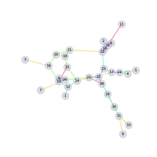
We used Networkx library for this, where each number is either a node or intersection with the colors corresponding to the length of the section of drawing connecting the nodes.
为此,我们使用了Networkx库,其中每个数字要么是一个节点,要么是与连接节点的工程图截面长度相对应的颜色的交点。
翻译自: https://towardsdatascience.com/classifying-parkinsons-disease-through-image-analysis-2e7a152fafc9
帕金森定律