2.Node Classification with Graph Neural Networks

       This tutorial will teach you how to apply Graph Neural Networks (GNNs) to the task of node classification.
       Here, we are given the ground-truth labels of only a small subset of nodes, and want to infer the labels for all the remaining nodes (transductive learning).

       Transductive learning是一种机器学习方法，它旨在通过使用现有的有标记数据来预测未标记数据的标签。具体来说，它是在仅考虑给定的一组训练数据和一组测试数据的情况下，尝试为测试数据分配标签的方法。
       与传统的监督学习不同，它不会为测试数据集中的每个实例都学习一个模型，而是尝试通过利用训练数据的上下文来生成一个全局模型，该模型可以为测试数据集中的所有实例预测标签。
       因此，transductive learning 可以在某些情况下对于特定任务比传统的监督学习方法更有效。但需要注意的是，transductive learning需要在测试集上进行训练，因此可能会对测试集数据过拟合，因此需要谨慎使用。

       To demonstrate, we make use of the Cora dataset, which is a citation network where nodes represent documents.
       Each node is described by a 1433-dimensional bag-of-words feature vector.Two documents are connected if there exists a citation link between them.The task is to infer the category of each document (7 in total).

       This dataset was first introduced by Yang et al. (2016) as one of the datasets of the Planetoid benchmark suite.
       We again can make use PyTorch Geometric for an easy access to this dataset via torch_geometric.datasets.Planetoid:

from torch_geometric.datasets import Planetoid
from torch_geometric.transforms import NormalizeFeatures

dataset = Planetoid(root='data/Planetoid', name='Cora', transform=NormalizeFeatures())

# NormalizeFeatures()是一种数据预处理技术，用于规范化特征值（即数据的列），以使它们具有相似的数值范围和分布。
# 这个函数的作用是将数据的每个特征值（或每一列）按照某种标准进行缩放和平移，使得它们的均值为0，方差为1，
# 这样可以使得不同特征之间具有可比性，避免由于特征值范围不同而对模型的训练造成影响。

# 在数据预处理阶段，使用NormalizeFeatures()可以帮助提高模型的性能，尤其是当特征值之间的尺度差异很大时，
# 如某些特征的值范围在千位或万位，而另一些特征的值范围只在十位或百位时，模型容易受到值范围大的特征的影响，
# 而无法充分利用其他特征的信息。因此，在使用机器学习算法之前，规范化特征值通常是一个必要的步骤。

print()
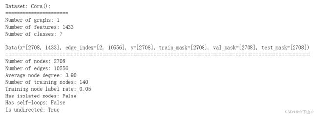
print(f'Dataset: {dataset}:')
print('======================')
print(f'Number of graphs: {len(dataset)}')
print(f'Number of features: {dataset.num_features}')
print(f'Number of classes: {dataset.num_classes}')

data = dataset[0]  # Get the first graph object.

print()
print(data)
print('===========================================================================================================')

# Gather some statistics about the graph.
print(f'Number of nodes: {data.num_nodes}')
print(f'Number of edges: {data.num_edges}')
print(f'Average node degree: {data.num_edges / data.num_nodes:.2f}')
print(f'Number of training nodes: {data.train_mask.sum()}')
print(f'Training node label rate: {int(data.train_mask.sum()) / data.num_nodes:.2f}')
print(f'Has isolated nodes: {data.has_isolated_nodes()}')
print(f'Has self-loops: {data.has_self_loops()}')
print(f'Is undirected: {data.is_undirected()}')

       Overall, this dataset is quite similar to the previously used KarateClub network.
       We can see that the Cora network holds 2,708 nodes and 10,556 edges, resulting in an average node degree of 3.9.
       For training this dataset, we are given the ground-truth categories of 140 nodes (20 for each class).
       This results in a training node label rate of only 5%.

       In contrast to KarateClub, this graph holds the additional attributes val_mask and test_mask, which denotes which nodes should be used for validation and testing.
       Furthermore, we make use of data transformations via transform=NormalizeFeatures().
       Transforms can be used to modify your input data before inputting them into a neural network, e.g., for normalization or data augmentation.
       Here, we row-normalize the bag-of-words input feature vectors.

       We can further see that this network is undirected, and that there exists no isolated nodes (each document has at least one citation).

Training a Multi-layer Perception Network (MLP)

       In theory, we should be able to infer the category of a document solely based on its content, i.e. its bag-of-words feature representation, without taking any relational information into account.

       Let’s verify that by constructing a simple MLP that solely operates on input node features (using shared weights across all nodes):

import torch
from torch.nn import Linear
import torch.nn.functional as F


class MLP(torch.nn.Module):
    def __init__(self, hidden_channels):
        super().__init__()
        torch.manual_seed(12345)
        self.lin1 = Linear(dataset.num_features, hidden_channels)
        self.lin2 = Linear(hidden_channels, dataset.num_classes)

    def forward(self, x):
        x = self.lin1(x)
        x = x.relu()
        x = F.dropout(x, p=0.5, training=self.training)
        
#         这段代码是在PyTorch中使用的，用于在神经网络中应用dropout正则化技术。
#         它通常被用于每个层的输入，可以有效减少过拟合风险，提高模型泛化能力。
#         对于给定的输入张量x，F.dropout()函数会根据给定的概率p随机将一些元素置为0，
#         并将剩余元素的值除以(1-p)，以保持元素的期望值不变。
#         同时，它还会检查模型是否处于训练模式，只在训练模式下应用dropout，
#         而在测试模式下不应用，这是为了避免测试过程中结果的不确定性。
#         因此，对于每个层的输入，通常会应用dropout操作来增强模型的泛化能力。
#         这是一个常用的正则化技术，可以有效地避免过拟合，并提高模型在新数据上的预测性能。
        
        x = self.lin2(x)
        return x

model = MLP(hidden_channels=16)
print(model)

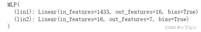
       Our MLP is defined by two linear layers and enhanced by ReLU non-linearity and dropout.
       Here, we first reduce the 1433-dimensional feature vector to a low-dimensional embedding (hidden_channels=16), while the second linear layer acts as a classifier that should map each low-dimensional node embedding to one of the 7 classes.

       Let’s train our simple MLP by following a similar procedure as described in the first part of this tutorial.
       We again make use of the cross entropy loss and Adam optimizer.
       This time, we also define a test function to evaluate how well our final model performs on the test node set (which labels have not been observed during training).

model = MLP(hidden_channels=16)
criterion = torch.nn.CrossEntropyLoss()  # Define loss criterion.
optimizer = torch.optim.Adam(model.parameters(), lr=0.01, weight_decay=5e-4)  # Define optimizer.

def train():
    model.train()
    optimizer.zero_grad()  # Clear gradients.
    out = model(data.x)  # Perform a single forward pass.
    loss = criterion(out[data.train_mask], data.y[data.train_mask])  # Compute the loss solely based on the training nodes.
    loss.backward()  # Derive gradients.
    optimizer.step()  # Update parameters based on gradients.
    return loss

def test():
    model.eval()
    out = model(data.x)
    pred = out.argmax(dim=1)  # Use the class with highest probability.
    test_correct = pred[data.test_mask] == data.y[data.test_mask]  # Check against ground-truth labels.
    test_acc = int(test_correct.sum()) / int(data.test_mask.sum())  # Derive ratio of correct predictions.
    return test_acc

for epoch in range(201):
    loss = train()
    if epoch % 40 == 0:
        print(f'Epoch: {epoch:03d}, Loss: {loss:.4f}')
        
test_acc = test()
print(f'Test Accuracy: {test_acc:.4f}')

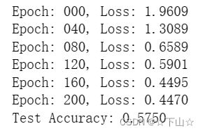
       As one can see, our MLP performs rather bad with only about 59% test accuracy.
       But why does the MLP do not perform better?
       The main reason for that is that this model suffers from heavy overfitting due to only having access to a small amount of training nodes, and therefore generalizes poorly to unseen node representations.

       It also fails to incorporate an important bias into the model: Cited papers are very likely related to the category of a document.
       That is exactly where Graph Neural Networks come into play and can help to boost the performance of our model.

Training a Graph Neural Network (GNN)

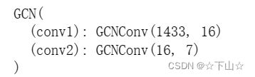
       We can easily convert our MLP to a GNN by swapping the torch.nn.Linear layers with PyG’s GNN operators.
       Following-up on the first part of this tutorial, we replace the linear layers by the GCNConv module.
       To recap, the GCN layer (Kipf et al. (2017)) is defined as

$${\mathbf{x}}_v^{(\ell +1)}={\mathbf{W}}^{(\ell +1)}\sum _{w\in \mathcal{N}(v)\cup \{v\}}\frac{1}{c_{w,v}}\cdot {\mathbf{x}}_w^{(\ell )}$$

       where ${\mathbf{W}}^{(\ell +1)}$ denotes a trainable weight matrix of shape [num_output_features, num_input_features] and $c_{w,v}$ refers to a fixed normalization coefficient for each edge.
       In contrast, a single Linear layer is defined as

$${\mathbf{x}}_v^{(\ell +1)}={\mathbf{W}}^{(\ell +1)}{\mathbf{x}}_v^{(\ell )}$$

       which does not make use of neighboring node information.

from torch_geometric.nn import GCNConv


class GCN(torch.nn.Module):
    def __init__(self, hidden_channels):
        super().__init__()
        torch.manual_seed(1234567)
        self.conv1 = GCNConv(dataset.num_features, hidden_channels)
        self.conv2 = GCNConv(hidden_channels, dataset.num_classes)

    def forward(self, x, edge_index):
        x = self.conv1(x, edge_index)
        x = x.relu()
        x = F.dropout(x, p=0.5, training=self.training)
        x = self.conv2(x, edge_index)
        return x

model = GCN(hidden_channels=16)
print(model)

       Let’s visualize the node embeddings of our untrained GCN network.
       For visualization, we make use of TSNE to embed our 7-dimensional node embeddings onto a 2D plane.

# Helper function for visualization.
%matplotlib inline
import matplotlib.pyplot as plt
from sklearn.manifold import TSNE

def visualize(h, color):
    z = TSNE(n_components=2, init='pca', learning_rate='auto').fit_transform(h.detach().cpu().numpy()) # 使用TSNE算法对该NumPy数组进行降维，将其从高维空间（h张量的维度）转换为一个二维空间
    # fit_transform函数会首先使用fit方法对数据进行拟合，然后使用transform方法将数据转换为降维后的特征表示
    print(z.shape)

    plt.figure(figsize=(10,10))
    plt.xticks([])
    plt.yticks([])

    plt.scatter(z[:, 0], z[:, 1], s=70, c=color, cmap="Set2")
    plt.show()

model = GCN(hidden_channels=16)
model.eval()

out = model(data.x, data.edge_index)
print(out.shape)

visualize(out, color=data.y)

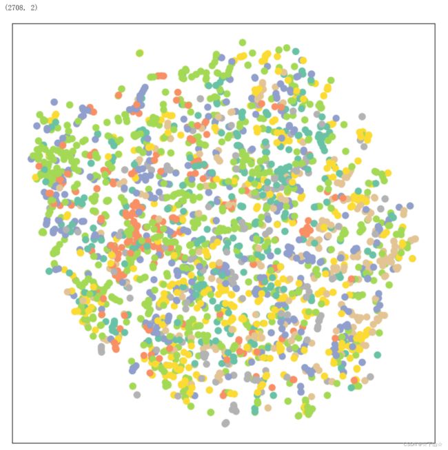
       We certainly can do better by training our model.
       The training and testing procedure is once again the same, but this time we make use of the node features x and the graph connectivity edge_index as input to our GCN model.

model = GCN(hidden_channels=16)
optimizer = torch.optim.Adam(model.parameters(), lr=0.01, weight_decay=5e-4)
criterion = torch.nn.CrossEntropyLoss()

def train():
    model.train()
    optimizer.zero_grad()  # Clear gradients.
    out = model(data.x, data.edge_index)  # Perform a single forward pass.
    loss = criterion(out[data.train_mask], data.y[data.train_mask])  # Compute the loss solely based on the training nodes.
    loss.backward()  # Derive gradients.
    optimizer.step()  # Update parameters based on gradients.
    return loss

def test():
    model.eval()
    out = model(data.x, data.edge_index)
    pred = out.argmax(dim=1)  # Use the class with highest probability.
    test_correct = pred[data.test_mask] == data.y[data.test_mask]  # Check against ground-truth labels.
    test_acc = int(test_correct.sum()) / int(data.test_mask.sum())  # Derive ratio of correct predictions.
    return test_acc


for epoch in range(101):
    loss = train()
    if epoch % 20 == 0:
        print(f'Epoch: {epoch:03d}, Loss: {loss:.4f}')
        
test_acc = test()
print(f'Test Accuracy: {test_acc:.4f}')

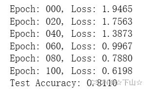
       There it is!
       By simply swapping the linear layers with GNN layers, we can reach 81.5% of test accuracy!
       This is in stark contrast to the 59% of test accuracy obtained by our MLP, indicating that relational information plays a crucial role in obtaining better performance.

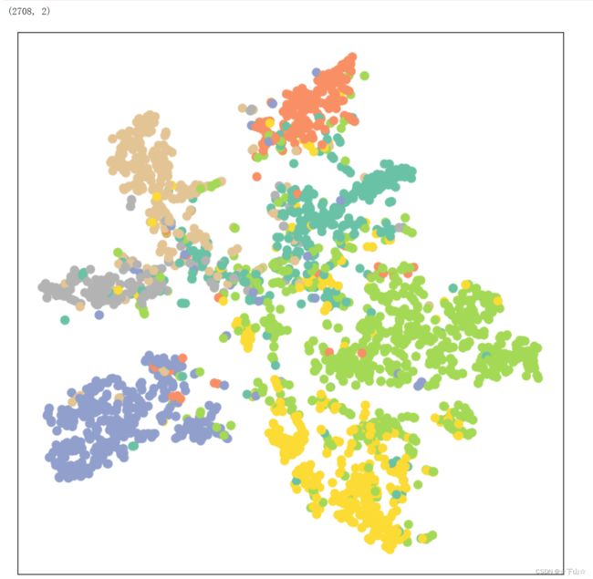
       We can also verify that once again by looking at the output embeddings of our trained model, which now produces a far better clustering of nodes of the same category.

model.eval()

out = model(data.x, data.edge_index)
visualize(out, color=data.y)

Conclusion

       In this chapter, you have seen how to apply GNNs to real-world problems, and, in particular, how they can effectively be used for boosting a model’s performance.

本文内容参考：PyG官网