gismo-3维IGA

---

前言

只是为方便学习，不做其他用途！

一、简单示例

参考网页 Tutorial 02: Geometry

#include 

using namespace gismo;

int main(int, char**)
{
    gsInfo.precision(3);
    gsKnotVector<>   kv(-1, 0, 3, 3, 1);
    gsBSplineBasis<> bsp(kv);
    gsInfo << bsp.detail() << "\n";

    bsp.uniformRefine();
    gsInfo << bsp.detail() << "\n";

    return 0;
}

二、gismo-3维IGA

运行代码需要配置好gismo环境
还需要将 terrific.xml 放在项目文件下，和cpp文件放在同一文件路径下

/// This is an example of using the linear elasticity solver on a 3D multi-patch geometry.
/// The problems is part of the EU project "Terrific".
///
/// Authors: O. Weeger (2012-1015, TU Kaiserslautern),
///          A.Shamanskiy (2016 - ...., TU Kaiserslautern)
#include 
#include 
#include 
#include 

using namespace gismo;

int main(int argc, char* argv[])
{
    gsInfo << "Testing the linear elasticity solver in 3D-线弹性求解器的三维测试.\n";

    //=============================================================//
                       // Input //
    //=============================================================//

    //std::string filename("terrific.xml");//初始数据文件
    std::string filename("test.xml");//初始数据文件
    real_t youngsModulus = 74e9;//杨氏模量
    real_t poissonsRatio = 0.33;//泊松比
    index_t numUniRef = 0;//节点插入数
    index_t numDegElev = 0;//升阶次数
    index_t numPlotPoints = 10000;//preview软件画图的点数量


    // minimalistic user interface for terminal 终端最简用户界面
    gsCmdLine cmd("Testing the linear elasticity solver in 3D.");// 定义一个gsCmdLine类 命名为cmd
    cmd.addInt("r", "refine", "Number of uniform refinement application", numUniRef);
    cmd.addInt("d", "degelev", "Number of degree elevation application", numDegElev);
    cmd.addInt("p", "points", "Number of points to plot to Paraview", numPlotPoints);
    try { cmd.getValues(argc, argv); } //  不太用看  不知道这个命令代表啥
    catch (int rv) { return rv; }

    //=====================================================================//
        // Scanning geometry and creating bases:扫描几何和创建基函数  //
    //=====================================================================//

    // scanning geometry 扫描几何
    gsMultiPatch<> geometry; //  定义一个多片
    gsReadFile<>(filename, geometry);// 将plateWithHole.xml文件中的数据赋值给 geometry
    // creating basis 生成基函数
    gsMultiBasis<> basis(geometry);
    for (index_t i = 0; i < numDegElev; ++i) // 升阶次数
        basis.degreeElevate();
    for (index_t i = 0; i < numUniRef; ++i) // k细化（节点插入）次数
        basis.uniformRefine();
    gsInfo << basis ;

    //=====================================================================//
        // Setting loads and boundary conditions  设置载荷和边界条件 //
    //=====================================================================//

    // source function, rhs  源函数？-解析解？
    gsConstantFunction<> f(0., 0., 0., 3);
    // surface load, neumann BC 黎曼边界对应载荷边界条件  荷载BC   力的边界条件
    gsConstantFunction<> g(20e6, -14e6, 0, 3);

    // boundary conditions 边界条件  黎曼边界对应载荷边界条件    dirichlete对应位移边界条件
    gsBoundaryConditions<> bcInfo;
    // Dirichlet BC are imposed separately for every component (coordinate) 对每个分量(坐标)分别施加 Dirichlet BC
    for (index_t d = 0; d < 3; d++)
    {
        bcInfo.addCondition(0, boundary::back, condition_type::dirichlet, 0, d);
       /* bcInfo.addCondition(1, boundary::back, condition_type::dirichlet, 0, d);
        bcInfo.addCondition(2, boundary::south, condition_type::dirichlet, 0, d);*/
    }
    // Neumann BC are imposed as one function 将 Neumann BC 作为一个函数
    bcInfo.addCondition(0, boundary::front, condition_type::neumann, &g);
    //bcInfo.addCondition(14, boundary::north, condition_type::neumann, &g);

    //=====================================================================//
              // Assembling & solving //
    //=====================================================================//

    // creating assembler   创建刚度矩阵?
    gsElasticityAssembler<real_t> assembler(geometry, basis, bcInfo, f);
    assembler.options().setReal("YoungsModulus", youngsModulus);
    assembler.options().setReal("PoissonsRatio", poissonsRatio);
    assembler.options().setInt("DirichletValues", dirichlet::l2Projection);
    gsInfo << "Assembling...\n";
    gsStopwatch clock;
    clock.restart();
    assembler.assemble();
    gsInfo << "Assembled a system with "
        << assembler.numDofs() << " dofs in " << clock.stop() << "s.\n";

    gsInfo << "Solving...\n";
    clock.restart();

#ifdef GISMO_WITH_PARDISO
    gsSparseSolver<>::PardisoLDLT solver(assembler.matrix());
    gsVector<> solVector = solver.solve(assembler.rhs());
    gsInfo << "Solved the system with PardisoLDLT solver in " << clock.stop() << "s.\n";
#else
    gsSparseSolver<>::SimplicialLDLT solver(assembler.matrix());
    gsVector<> solVector = solver.solve(assembler.rhs());
    gsInfo << "Solved the system with EigenLDLT solver in " << clock.stop() << "s.\n";
#endif

    //=====================================================================//
                  // Output //
    //=====================================================================//

    // constructing solution as an IGA function
    gsMultiPatch<> solution;
    assembler.constructSolution(solVector, assembler.allFixedDofs(), solution);
    // constructing stresses
    gsPiecewiseFunction<> stresses;
    assembler.constructCauchyStresses(solution, stresses, stress_components::von_mises);

    if (numPlotPoints > 0)
    {
        // constructing an IGA field (geometry + solution)
        gsField<> solutionField(assembler.patches(), solution);
        gsField<> stressField(assembler.patches(), stresses, true);
        // creating a container to plot all fields to one Paraview file
        std::map<std::string, const gsField<>*> fields;
        fields["Deformation"] = &solutionField;
        fields["von Mises"] = &stressField;
        gsWriteParaviewMultiPhysics(fields, "test_le", numPlotPoints);
        gsInfo << "Open \"test_le.pvd\" in Paraview for visualization.\n";
    }

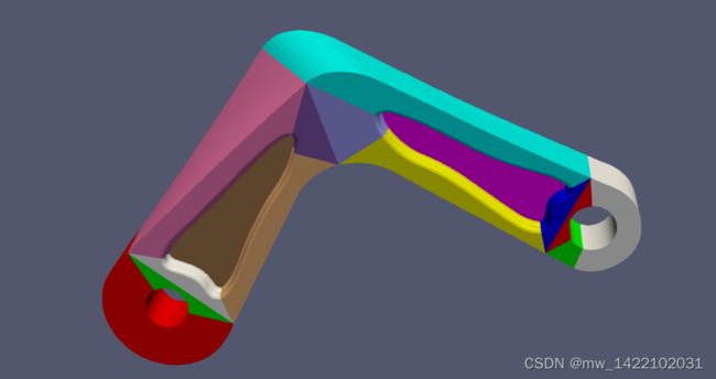
    return 0;
}

3维程序中的几何模型

三、xml文件的理解

1、xml文件示例

网址https://gismo.github.io/Tutorial02.html

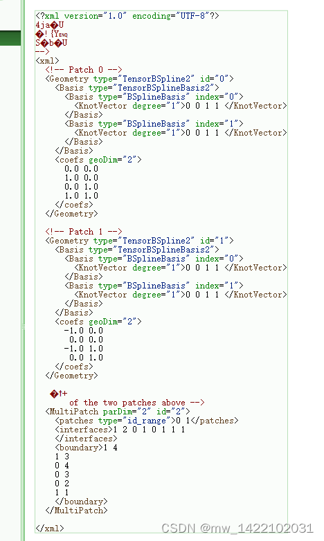
2、gismo中二维示例文件-一个曲面（简单）

可以参考之前的博客gismo中用等几何解决线弹性问题的程序示例来理解xml文件

注： 一个平面没有 interfaces这一项
对 interfaces这一项 目前还没有理解

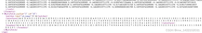
四、三维程序中xml文件的理解

三维几何模型

边界信息

给的示例文件中有15个体组装在一起

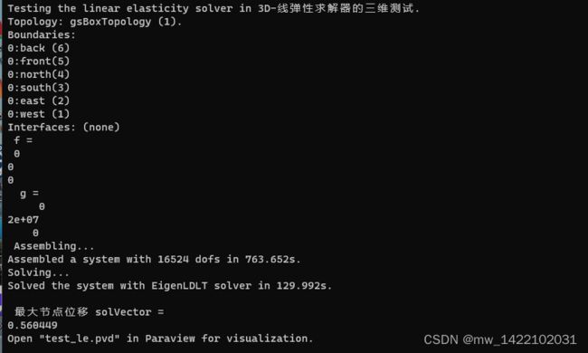
五、三维程序运行

细化四次

运行时间：14分钟

细化5次

运行时间：4.58h
组总刚：1.6h
解方程组：2.98h

总结 #pic_center

空格         空格

：

二维数

1

1

1