有向图 寻路算法
旅游旅客 (Traveling tourist)
In the first part of the series, we constructed a knowledge graph of monuments located in Spain from WikiData API. Now we’ll put on our graph data science goggles and explore various pathfinding algorithms available in the Neo4j Graph Data Science library. To top it off, we’ll look at a brute force solution for a Santa Claus problem. Now, you might wonder what a Santa Claus problem is. It is a variation of the traveling salesman problem, except we don’t require the solution to end in the same city as it started. This is because of the Santa Claus’ ability to bend the time-space continuum and instantly fly back to the North Pole once he’s finished with delivering goodies.
在本系列的第一部分中 ,我们从WikiData API构建了位于西班牙的古迹的知识图。 现在,我们将穿上我们的图形数据科学护目镜,并探索Neo4j图形数据科学库中可用的各种寻路算法。 最重要的是,我们将研究针对圣诞老人问题的蛮力解决方案。 现在,您可能想知道圣诞老人的问题是什么。 这是旅行商问题的一个变体,除了我们不要求解决方案在开始时所在的城市结束。 这是因为圣诞老人能够弯曲时空连续体,并在他完成交付好东西后立即飞回北极。
议程 (Agenda)
- Infer spatial network of monuments 推断古迹的空间网络
- Load the in-memory projected graph with cypher projection 使用密码投影加载内存中投影图
- Weakly connected component algorithm 弱连接组件算法
- Shortest path algorithm 最短路径算法
- Yen’s k-shortest path algorithm 日元的K最短路径算法
- Single source shortest paths algorithm 单源最短路径算法
- Minimum spanning tree algorithm 最小生成树算法
- Random walk algorithm 随机游走算法
- Traveling salesman problem 旅行商问题
- Conclusion 结论
推断古迹的空间网络 (Infer spatial network of monuments)
Currently, we have no direct relationships between the monuments in our graph. We do, however, have their GPS locations, which allows us to identify which monuments are nearby. This way, we can infer a spatial network of monuments.
目前,我们的图表中的纪念碑之间没有直接关系。 但是,我们确实拥有其GPS位置,这使我们能够识别附近有哪些古迹。 这样,我们可以推断出古迹的空间网络。
The process is very similar to inferring a similarity network. We usually don’t want to end up with a complete graph, where each node is connected to all the other ones. It would defeat the purpose of demonstrating pathfinding algorithms as the shortest path between any two nodes would always be a straight line, which would be represented as a direct relationship between the two nodes. In our case, we will connect each monument to the five closest monuments that are less than 100 kilometers away. These two numbers are entirely arbitrary. You can pick any other depending on your scenario.
该过程与推断相似性网络非常相似。 我们通常不希望最终得到一个完整的图,其中每个节点都与所有其他节点相连。 由于任何两个节点之间的最短路径始终是一条直线,因此将无法证明演示寻路算法的目的,这将被表示为两个节点之间的直接关系。 在我们的案例中,我们会将每个纪念碑与距离最近的100个距离不到的五座纪念碑相连。 这两个数字完全是任意的。 您可以根据情况选择其他任何一种。
MATCH (m1:Monument),(m2:Monument)
WHERE id(m1) > id(m2)
WITH m1,m2, distance(m1.location_point,m2.location_point) as distance
ORDER BY distance ASC
WHERE distance < 100000
WITH m1,collect({node:m2,distance:distance})[..5] as nearest
UNWIND nearest as near
WITH m1, near, near.node as nearest_node
MERGE (m1)-[m:NEAR]-(nearest_node) SET m.distance = near.distance
使用密码投影加载内存中投影图 (Load the in-memory projected graph with cypher projection)
Let’s just quickly refresh how does the GDS library work.
让我们快速刷新一下GDS库的工作方式。
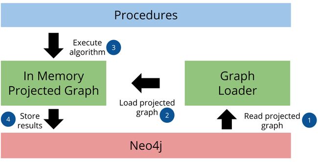
official documentation. 官方文档中借用的。The graph analytics pipeline consists of three parts. In the first part, the graph loader reads the stored graph from Neo4j and loads it as an in-memory projected graph. We can use either native projection or cypher projection to load the projected graph. In the second step, we execute the graph algorithms in sequence. We can use the results of one graph algorithm as an input to another. Last but not least, we store or stream the results back to Neo4j.
图分析管道包括三个部分。 在第一部分中,图加载器从Neo4j中读取存储的图,并将其作为内存中的投影图加载。 我们可以使用本机投影或密码投影来加载投影图。 在第二步中,我们依次执行图算法。 我们可以将一种图形算法的结果用作另一种图形算法的输入。 最后但并非最不重要的一点是,我们将结果存储或流回Neo4j。
Here, we will use the cypher projection to load the in-memory graph. I suggest you take a look at the official documentation for more details regarding how it works. In the node statement, we will describe all monuments in our graph and add their architecture style as a node label. Adding a custom node label will allow us to filter nodes by architectural style at algorithm execution time. In the relationship statement, we will describe all the links between monuments and include the distance property, that we will use as a relationship weight.
在这里,我们将使用密码投影来加载内存中的图。 我建议您查看官方文档,以获取有关其工作原理的更多详细信息。 在node语句中,我们将在图中描述所有纪念碑,并将其建筑风格添加为node标签。 添加自定义节点标签将使我们能够在算法执行时按体系结构样式过滤节点。 在关系声明中,我们将描述纪念碑之间的所有链接,并包括distance属性,将其用作关系权重。
CALL gds.graph.create.cypher('monuments',
  'MATCH (m:Monument)-[:ARCHITECTURE]->(a)
   RETURN id(m) as id, collect(a.name) as labels',
  'MATCH (m1:Monument)-[r:NEAR]-(m2:Monument)
   RETURN id(m1) as source, id(m2) as target, r.distance as distance')
弱连接组件算法 (Weakly connected component algorithm)
Even though the weakly connected component algorithm is not a pathfinding algorithm, it is part of almost every graph analysis. It is used to find disconnected components or islands within our graph. We’ll begin by running the stats mode of the algorithm.
即使弱连接组件算法不是寻路算法,它也几乎是每个图形分析的一部分。 它用于查找图中的断开连接的组件或孤岛。 我们将从运行算法的stats模式开始。
CALL gds.wcc.stats('monuments')
YIELD componentCount, componentDistribution
Results
结果
There are six separate components within our monuments network. The results are typical for a real-world dataset. We have a single super component that contains 98% of all nodes and a couple of tiny islands floating around. Let’s examine the smaller components.
我们的古迹网络包含六个独立的组件。 结果是真实数据集的典型结果。 我们只有一个超级组件,其中包含98%的所有节点以及几个漂浮的小岛。 让我们研究一下较小的组件。
CALL gds.wcc.stream('monuments')
YIELD nodeId, componentId
WITH componentId, gds.util.asNode(nodeId) as node
OPTIONAL MATCH (node)-[:IS_IN*2..2]->(state)
RETURN componentId,
       count(*) as component_size,
       collect(node.name) as monuments,
       collect(distinct state.id) as state
ORDER BY component_size DESC
SKIP 1
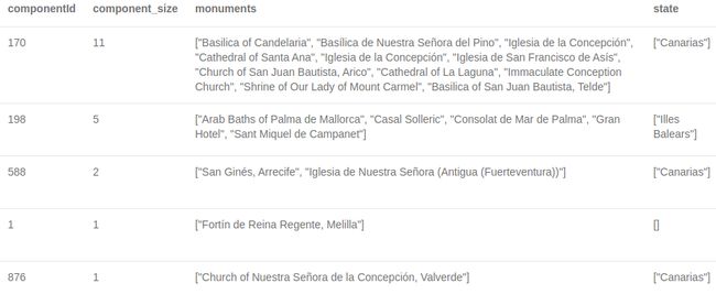
Results
结果
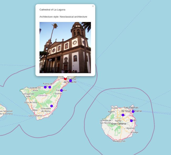
Smaller weakly connected components members 较小的弱连接组件成员Three of the five smaller components are located in the Canaries archipelago, and one is located in the Balearic Islands, specifically on Majorca. With the Neomap application, developed by Estelle Scifo, we can visualize the Canaries archipelago components on a map.
五个较小的组成部分中的三个位于加那利群岛,一个位于巴利阿里群岛,特别是在马略卡岛。 使用Estelle Scifo开发的Neomap应用程序 ,我们可以在地图上可视化Canaries群岛组件。
One component spans over two monuments on Fuerteventura and Lanzarote. The second one consists of a couple of monuments located on Tenerife and Gran Canaria. On the left, there is a single monument on El Hierro Island. They are separate components because there is no link between them. The absence of a connection between the components implies that there are more than 100 kilometers away because that is the threshold we chose when we inferred the spatial network.
一个组成部分跨越了费埃特文图拉岛和兰萨罗特岛上的两个纪念碑。 第二个由在特内里费岛和大加那利岛上的几个纪念碑组成。 左侧是耶罗岛上的单个纪念碑。 它们是独立的组件,因为它们之间没有链接。 组件之间没有连接意味着相距100多公里,因为这是我们推断空间网络时选择的阈值。
P.s. If you like any water activities, I highly recommend visiting the Canaries.
附言:如果您喜欢任何水上活动,我强烈建议您参观金丝雀。
最短路径算法 (Shortest Path algorithm)
The first pathfinding graph algorithm we will use is the Shortest Path algorithm. It finds the shortest weighted path between two nodes. We define the start node and the end node and specify which relationship weight property should the algorithm take into consideration when calculating the shortest path.
我们将使用的第一个寻路图算法是最短路径算法 。 它找到两个节点之间的最短加权路径。 我们定义起点和终点,并指定算法在计算最短路径时应考虑的关系权重属性。
MATCH (s:Monument{name:'Iglesia de Santo Domingo'}),
      (e:Monument{name:'Colegiata de Santa María de Piasca'})
CALL gds.alpha.shortestPath.stream('monuments',{
  startNode:s,
  endNode:e,
  relationshipWeightProperty:'distance'})
YIELD nodeId, cost
RETURN gds.util.asNode(nodeId).name as monument, cost
Results
结果
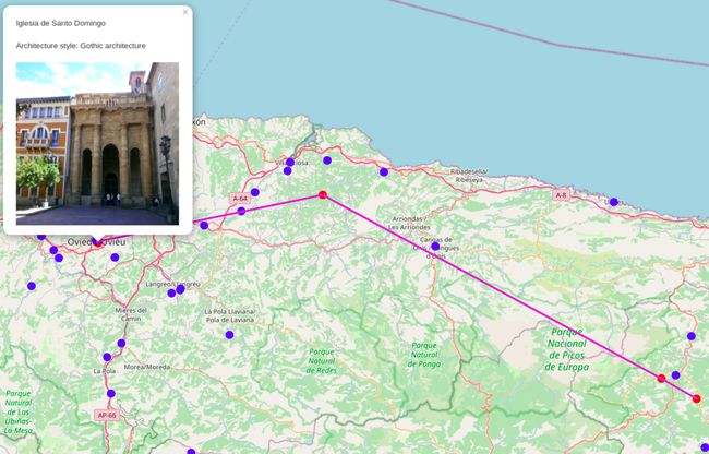
The cost is expressed as the distance in meters. We can visualize the shortest path with a slightly modified version of Neomap. I have customized the popup of the monuments to include its image and the architectural style.
成本表示为以米为单位的距离。 我们可以通过稍微修改版本的Neomap来可视化最短路径。 我自定义了纪念碑的弹出窗口,以包括其图像和建筑风格。
You might observe that we skip the Santa Cruz de Cangas de Onís monument, which is located in the middle right of the image. A slight detour will result in a longer path than just traversing in a straight line from Iglesia de San Emeterio to Santo Toribio de Liébana.
您可能会发现,我们跳过了位于图像右中角的Santa Cruz de Cangas deOnís纪念碑。 略微走弯比从Iglesia de San Emeterio到Santo Toribio deLiébana直线行驶的路径更长。
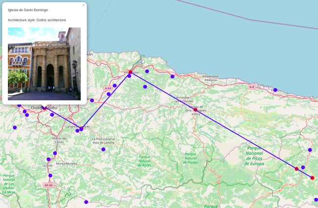
What if we wanted to plan a trip for an architectural class and visit only monuments that were influenced by either Gothic or Romanesque architecture along the way? Planning such a trip is very easy with the GDS library, as we can filter which nodes can the algorithm visit with the nodeLabels parameter.
如果我们想计划一次建筑课程的旅行,并只参观沿途受到哥特式或罗马式建筑影响的纪念碑,该怎么办? 使用GDS库非常容易计划这样的行程,因为我们可以使用nodeLabels参数过滤算法可以访问哪些节点。
MATCH (s:Monument{name:'Iglesia de Santo Domingo'}),
      (t:Monument{name:'Colegiata de Santa María de Piasca'})
CALL gds.alpha.shortestPath.stream('monuments',{
  startNode:s,
  endNode:t,
  relationshipWeightProperty:'distance',
  nodeLabels:['Gothic architecture','Romanesque architecture']})
YIELD nodeId, cost
RETURN gds.util.asNode(nodeId).name as monument, cost
Results
结果
The route is a bit different this time as the algorithm can only visit monuments that were influenced by Gothic or Romanesque architecture style.
这次的路线有所不同,因为该算法只能访问受哥特式或罗马式建筑风格影响的纪念碑。
日元的K最短路径算法 (Yen’s k-shortest path algorithm)
We have learned how to calculate the shortest weighted path between a pair of nodes. What if we were more cautious tourists and wanted to find the top three shortest paths? Having a backup plan if something unexpected might happen along the way is always a good idea. In this scenario, we could use the Yen’s k-shortest path algorithm. The syntax is almost identical to the Shortest Path algorithm, except for the added k parameter, which defines how many shortest paths we would like to find.
我们已经学习了如何计算一对节点之间的最短加权路径。 如果我们是比较谨慎的游客,并且想找到最短的前三条路线怎么办? 如果在此过程中可能发生意外,制定备份计划始终是一个好主意。 在这种情况下,我们可以使用日元的k最短路径算法 。 除了添加的k参数(定义了我们希望查找多少条最短路径)外,语法几乎与最短路径算法相同。
MATCH (s:Monument{name:'Iglesia de Santo Domingo'}),
      (t:Monument{name:'Colegiata de Santa María de Piasca'})
CALL gds.alpha.kShortestPaths.stream('monuments',{
  startNode:s,
  endNode:t,
  k:3,
  relationshipWeightProperty:'distance'})
YIELD index,nodeIds,costs
RETURN index,[nodeId in nodeIds | gds.util.asNode(nodeId).name] as monuments,apoc.coll.sum(costs) as total_cost
Results
结果
Yen’s k-shortest path algorithm results 日元的k最短路径算法结果The three paths are almost the same length, just a couple hundred meters of difference. If you look closely, only the second stop is different among the three variants. Such a small difference can be attributed to the nature of our spatial network and the example pair of nodes.
这三个路径的长度几乎相同,相差仅几百米。 如果仔细观察,这三个变体之间只有第二个停靠点是不同的。 如此小的差异可以归因于我们的空间网络和示例节点对的性质。
单源最短路径算法 (Single source shortest path algorithm)
With the Single Source Shortest Path algorithm, we define the start node and search for the shortest weighted path to all the other nodes in the network. We’ll inspect one of the Canaries components to limit the number of shortest paths to a reasonable number.
使用“ 单源最短路径”算法 ,我们定义了起始节点,并搜索到网络中所有其他节点的最短加权路径。 我们将检查Canaries组件之一,以将最短路径的数量限制为合理的数量。
We’ll examine the Tenerife — Gran Canaria component and choose the Cathedral of La Laguna as the starting node. The algorithm tries to find the shortest paths to all the other nodes in the network, and if no such way exists, it returns Infinity value as a result. We will filter out the unreachable nodes with the gds.util.isFinite procedure.
我们将研究Tenerife-Gran Canaria组件,并选择La Laguna大教堂作为起始节点。 该算法尝试查找到网络中所有其他节点的最短路径,如果不存在这种方式,则结果将返回Infinity值。 我们将使用gds.util.isFinite过程过滤掉无法访问的节点。
MATCH (start:Monument{name:’Cathedral of La Laguna’})
CALL gds.alpha.shortestPaths.stream(‘monuments’,
 {startNode:start, relationshipWeightProperty:’distance’})
YIELD nodeId, distance
WHERE gds.util.isFinite(distance) = True
RETURN gds.util.asNode(nodeId).name as monument,distance
ORDER BY distance ASC
Results
结果
The closest monument to the Cathedral of La Laguna is the Iglesia de la Concepción, which is just 420 meters away. It seems that there are two Iglesia de la Concepción on Tenerife Island as we can observe that it shows up twice in our results. The farthest reachable monument in our network from the Cathedral of La Laguna is Basilica of San Juan Bautista.
最接近拉古纳大教堂的纪念碑是伊格莱西亚·德拉Kong塞普西翁(Iglesia de laConcepción),相距仅420米。 特内里费岛上似乎有两个Iglesia de laConcepción,因为我们可以看到它在我们的结果中显示了两次。 从拉古纳大教堂出发,我们网络中距离最远的纪念碑是圣胡安·包蒂斯塔大教堂。
If we wanted to find the cost of the shortest path to all the reachable neoclassical monuments from the Cathedral of La Laguna, we could effortlessly achieve this with the nodeLabels parameter.
如果我们想找到从拉古纳大教堂通往所有可到达的新古典主义古迹的最短路径的成本,则可以使用nodeLabels参数毫不费力地实现这一nodeLabels 。
MATCH (start:Monument{name:'Cathedral of La Laguna'})
CALL gds.alpha.shortestPaths.stream('monuments',
 {startNode:start, relationshipWeightProperty:'distance',
  nodeLabels:['Neoclassical architecture']})
YIELD nodeId, distance
WHERE gds.util.isFinite(distance) = True
RETURN gds.util.asNode(nodeId).name as monument,
 distance
ORDER BY distance ASC
Results
结果
It seems there are only four neoclassical monuments on Tenerife and Gran Canaria islands.
特内里费岛和大加那利岛上似乎只有四个新古典主义纪念碑。
最小权重生成树算法 (Minimum weight spanning tree algorithm)
The Minimum Weight Spanning Tree algorithm starts from a given node and calculates a spanning tree connecting all reachable nodes with the minimum possible sum of relationship weights. For example, if we wanted to connect all the monuments in Tenerife and Gran Canaria with an optical or electric cable, we would use the Minimum Weight Spanning Tree algorithm.
最小权重生成树算法从给定节点开始,并计算以所有关系权重的最小和连接所有可到达节点的生成树。 例如,如果我们想用光缆或电缆将特内里费岛和大加那利岛的所有古迹连接起来,则可以使用“最小重量生成树”算法。
MATCH (start:Monument{name:’Cathedral of La Laguna’})
CALL gds.alpha.spanningTree.minimum.write(‘monuments’,{
 startNodeId:id(start),
 relationshipWeightProperty:’distance’,
 weightWriteProperty:’cost’})
YIELD effectiveNodeCount
RETURN effectiveNodeCount
Results
结果
Currently, only the write mode of the algorithm is available. We can visualize our potential cable route with Neomap.
当前,仅算法的write模式可用。 我们可以使用Neomap可视化潜在的电缆路线。
随机游走算法 (Random walk algorithm)
We can imagine the Random Walk algorithm trying to mimic a drunk crowd traversing the network. They might go left, or right, take two steps forward, one step back, we never really know. It depends on how drunk the crowd is. We can use this algorithm to provide random trip recommendations. Imagine we have just visited the University of Barcelona historical building and are not sure which monuments we should take a look at next.
我们可以想象随机游走算法试图模仿醉酒的人群穿越网络。 他们可能向左走或向右走,向前走了两步,向后走了一步,我们从未真正知道。 这取决于人群有多醉。 我们可以使用此算法来提供随机行程建议。 想象一下,我们刚刚参观了巴塞罗那大学的历史建筑,并且不确定接下来应该参观哪些古迹。
MATCH (m:Monument{name:"University of Barcelona historical building"})
CALL gds.alpha.randomWalk.stream('monuments',
  {start:id(m), walks:3, steps:5})
YIELD nodeIds
RETURN [nodeId in nodeIds | gds.util.asNode(nodeId).name] as result
Results
结果
Remember, we mentioned that the Random Walk algorithm tries to mimic a drunk person traversing the network. Well, an intoxicated person might visit the same monument twice and not care. For example, in the first and third suggestions, a single monument shows up twice. Luckily, we have some options to influence how the algorithm should traverse the network in the node2vec mode with the following two parameters:
记住,我们提到随机游走算法试图模仿醉酒的人穿越网络。 好吧,一个醉酒的人可能会两次参观同一座古迹,而不在乎。 例如,在第一个和第三个建议中,单个纪念碑显示两次。 幸运的是,我们有一些选项可以影响该算法如何使用以下两个参数在node2vec模式下穿越网络:
return: This parameter controls the likelihood of immediately revisiting a node in a walk. Setting it to a high value (> max(inOut, 1)) ensures that we are less likely to sample an already visited node in the following two steps.
return:此参数控制立即重走行走中的节点的可能性。 将其设置为较高的值(> max(inOut,1))可确保我们在以下两个步骤中不太可能对已访问的节点进行采样。
inOut: This parameter allows the search to differentiate between “inward” and “outward” nodes. If inOut > 1, the random walk is biased towards nodes close to node t. In contrast, if inOut < 1, the walk is more inclined to visit nodes that are further away from the node t.
inOut:此参数允许搜索区分“向内”和“向外”节点。 如果inOut> 1,则随机游走会偏向靠近节点t的节点。 相反,如果inOut <1,则步行更倾向于访问距离节点t更远的节点。
The definition of the two parameters is summarized from the original Node2vec paper.
这两个参数的定义是从 原始Node2vec论文中 总结的 。
We want to recommend monuments close to our starting point, so we choose the inOut parameter to be greater than 1. And we definitely would like to avoid revisiting an already visited node during the walk, so we choose the return parameter to be greater than the inOut parameter.
我们想推荐靠近起点的纪念碑,因此我们选择inOut参数大于1。并且我们绝对希望避免在步行过程中重新访问已经访问过的节点,因此我们选择return参数大于inOut参数。
MATCH (m:Monument{name:"University of Barcelona historical building"})
CALL gds.alpha.randomWalk.stream('monuments',
  {start:id(m), walks:3, steps:5,
   mode:'node2vec', inOut:5, return:10})
YIELD nodeIds
RETURN [nodeId in nodeIds | gds.util.asNode(nodeId).name] as result
Results
结果
Unfortunately, the return parameter ensures that we are less likely to sample an already visited node in the following two steps. This means that we can’t be sure that duplicates won’t show up later during our walk. In our example, Casa Batlló appears twice in the first suggestion. We can circumnavigate this problem by creating longer walk suggestions and filtering out duplicates before showing the results to the user. In the following query, we calculate nine steps long walks, filter out duplicates, and return only the first five results.
不幸的是, return参数确保我们在以下两个步骤中不太可能对已经访问过的节点进行采样。 这意味着我们无法确定重复的内容不会在以后的步行过程中显示。 在我们的示例中,CasaBatlló在第一个建议中出现了两次。 我们可以通过创建更长的步行建议并在向用户显示结果之前过滤掉重复项来解决这个问题。 在下面的查询中,我们计算了九步走,筛选出重复项,仅返回前五个结果。
MATCH (m:Monument{name:"University of Barcelona historical building"})
CALL gds.alpha.randomWalk.stream('monuments',
  {start:id(m), walks:3, steps:9,
   mode:'node2vec', inOut:5, return:10})
YIELD nodeIds
RETURN apoc.coll.toSet([nodeId in nodeIds | gds.util.asNode(nodeId).name])[..5] as result
Results
结果
Random Walk algorithm results with removed duplicates 删除重复项的随机游走算法结果This way, we make sure the results never contain duplicates. Now we can visualize the results with our trip recommendation application.
这样,我们确保结果永远不会包含重复项。 现在,我们可以使用旅行推荐应用程序将结果可视化。
旅行商问题 (Traveling salesman problem)
To top it off, we will solve the Santa Claus variation of the traveling salesman problem. As mentioned, the only difference is that we omit the requirement to end up in the same location as we started. I found the inspiration for this problem in the Gaming the Christmas Market post written by David Barton. I give all the credits to David Barton for conjuring up the solution. My contribution is to update it to work with Neo4j 4.0 and the GDS library.
最重要的是,我们将解决旅行商问题的圣诞老人变化。 如前所述,唯一的区别是我们省略了与开始时位于同一位置的要求。 我在大卫·巴顿(David Barton)撰写的“ 游戏圣诞节市场”一文中找到了解决此问题的灵感。 我将所有荣誉归功于David Barton提出的解决方案。 我的贡献是将其更新为可与Neo4j 4.0和GDS库一起使用。
Say we want to find the optimal route between this monuments:
假设我们想找到这些纪念碑之间的最佳路线:
:param selection => ["Castell de Santa Pau","Castell de Sant Jaume","Castell de Vilaüt","Castell de Sarraí","Castell de Solius","Portal d'Albanyà","Castell de Sant Gregori","Casa Frigola"]We split the solution into two steps. First, we calculate the shortest path between all pairs of selected monuments with the gds.alpha.shortestPath algorithm and store the results as the SHORTEST_ROUTE_TO relationship between the given pair of nodes. We save the total cost and all the intermediate nodes along the shortest path as the properties of the SHORTEST_ROUTE_TO relationship.
我们将解决方案分为两个步骤。 首先,我们使用gds.alpha.shortestPath算法计算所有选定古迹对之间的最短路径,并将结果存储为给定节点对之间的SHORTEST_ROUTE_TO关系。 我们将总成本和沿最短路径的所有中间节点保存为SHORTEST_ROUTE_TO关系的属性。
WITH $selection as selection
MATCH (c:Monument)
WHERE c.name in selection
WITH collect(c) as monuments
UNWIND monuments as c1
WITH c1,
    [c in monuments where c.name > c1.name | c] as c2s,
    monuments
UNWIND c2s as c2
CALL gds.alpha.shortestPath.stream('monuments',{startNode:c1,endNode:c2,relationshipWeightProperty:'distance'})
YIELD nodeId, cost
WITH c1,
     c2,
     max(cost) as totalCost,
     collect(nodeId) as shortestHopNodeIds
MERGE (c1) -[r:SHORTEST_ROUTE_TO]- (c2)
SET r.cost = totalCost,
    r.shortestHopNodeIds = shortestHopNodeIds
After completing the first step, we have created a complete graph of SHORTEST_ROUTE_TO relationships between the selected monuments.
完成第一步后,我们创建了选定古迹之间的SHORTEST_ROUTE_TO关系的完整图形。
Traveling salesman problem step 1 旅行商问题第一步In the second step, we will use the apoc.path.expandConfig procedure. It enables us to perform variable-length path traversals with fine-grained control over the traversals. Check out the documentation for more details.
在第二步中,我们将使用apoc.path.expandConfig过程。 它使我们能够对遍历进行细粒度控制,从而执行变长路径遍历。 查看文档以获取更多详细信息。
We allow the procedure to traverse only SHORTEST_ROUTE_TO relationships with the relationshipFilter parameter and visit only the selected monuments with the whitelistNodes parameter. We ensure that all selected nodes must be visited exactly once by defining the number of hops or levels traversed (minLevel and maxLevel) and with the uniqueness parameter. I know it is a lot to comprehend, and if you need some help, I would suggest asking questions on the Neo4j community site. We then select the path with the minimum sum of relationship weights as the solution. Because we calculate all the possible routes between the chosen monuments, this is a brute-force solution of the traveling salesman problem.
我们允许该过程仅遍历带有relationshipFilter参数的SHORTEST_ROUTE_TO关系,并仅访问带有whitelistNodes参数的选定纪念碑。 我们确保所有选择的节点都必须通过定义跳或水平穿越(数量恰好一次访问minLevel和maxLevel ),并与uniqueness参数。 我知道您有很多了解,如果您需要帮助,我建议您在Neo4j社区网站上提问。 然后,我们选择关系权重最小的路径作为解决方案。 因为我们计算了选定古迹之间的所有可能路线,所以这是旅行商问题的蛮力解决方案。
WITH $selection as selection
MATCH (c:Monument)
WHERE c.name in selection
WITH collect(c) as monuments
UNWIND monuments as c1
WITH c1,
    [c in monuments where c.name > c1.name | c] as c2s,
    monuments,
    (size(monuments) - 1) as level
UNWIND c2s as c2
CALL apoc.path.expandConfig(c1, {
  relationshipFilter: 'SHORTEST_ROUTE_TO',
  minLevel: level,
  maxLevel: level,
  whitelistNodes: monuments,
  terminatorNodes: [c2],
  uniqueness: 'NODE_PATH'})
YIELD path
WITH path,
    reduce(cost = 0, x in relationships(path) | cost + x.cost) as totalCost
ORDER BY totalCost LIMIT 1
WITH path,
     totalCost,
     apoc.coll.flatten([r in relationships(path) | r.shortestHopNodeIds]) as intermediate_stops,
     [n in nodes(path) | id(n)] as node_ids
RETURN  [n in nodes(path) | n.name] as path,
        round(totalCost) as total_distance,
        [optional in intermediate_stops where not optional in node_ids | gds.util.asNode(optional).name] as optional_stops
Results
结果
Santa Claus solution 圣诞老人解决方案In the path column of the results, we have an ordered array of selected monuments to visit. Our travel would start with Castell de Sant Jaume and continue to Castell de Vilaüt and so on. We could dub this the Spanish castle-visiting trip as we selected six castles, and we have an option to see four more along the way. The total air distance of the path is 126 kilometers. Let’s visualize the results with our trip recommendation application.
在结果的路径栏中,我们有顺序排列的一组选定古迹供参观。 我们的旅行将从卡斯特尔·德·桑特·海姆出发,然后继续到卡斯特尔·德·维劳特,等等。 当我们选择六座城堡时,我们可以为这次西班牙城堡之旅做个配音,我们可以选择沿途再看四座。 该路径的总空中距离为126公里。 让我们通过旅行推荐应用程序来可视化结果。
Red markers are the selected monuments, and the blue markers are the optional stops along the way.
红色标记是选定的古迹,蓝色标记是沿途的可选站点。
结论 (Conclusion)
We have demonstrated most of the pathfinding algorithm available in the Neo4j Graph Data Science library with some real world use cases. The only puzzle left in this series is to finish the trip recommendation application. I have a plan to show off the application in the part three of the series. Till then, I encourage you to play around with various GDS library algorithm or try to recreate this series on a Neo4j sandbox instance. If you have any further questions, there are a bunch of Neo4j experts ready to help you on Neo4j community site.
我们已经在Neo4j Graph Data Science库中演示了大多数寻路算法,并提供了一些实际的用例。 本系列剩下的唯一难题是完成旅行推荐应用程序。 我计划在本系列的第三部分中展示该应用程序。 到那时,我鼓励您尝试各种GDS库算法,或者尝试在Neo4j沙箱实例上重新创建此系列。 如果您还有其他问题, Neo4j社区站点上将有很多Neo4j专家随时为您提供帮助。
As always, the code is available on GitHub.
与往常一样,该代码在GitHub上可用 。
翻译自: https://towardsdatascience.com/part-2-exploring-pathfinding-graph-algorithms-e194ffb7f569
有向图 寻路算法
