【无标题】

文本向量表示

文本的向量空间分为：
word-word (term-context)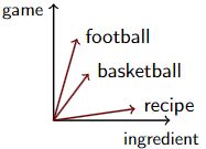

document-word (bag-of-words)

用向量表示文本的好处可能有：

• 对单词的含义进行编码，以便我们可以计算它们之间的语义相似度
• 方便进行文件检索，例如检索与查询相关的文档（网络搜索
• 将机器学习应用于文本数据，例如聚类/分类算法对向量进行操作。

Tokenisation 从原始文本中获取标记，最简单的方式：用空格拆分文本，用正则表达式，lowercasing,
punctuation/number/stop/infrequent word removal and stemming

常见的把文本变向量的方式：one-hot encoding，但是这个没有上下文之间的关系

Word-Word Matrix:
矩阵 X , n × m 其中 n = |V| （目标词）和 m = |Vc | （上下文词），对于 V 中的每个词 xi，计算它与上下文词 xj 共现的次数，使用 ±k 个单词的上下文窗口（在 xi 的左/右）。计算大量文档频率。
通常目标词和上下文词词汇表是相同的，结果是一个方阵

对文本的常用词向量，可以用加权处理：
vocabulary = [aadvark, computer, data, pinch, result, sugar, the]
apricot = x2 = [0, 0, 0, 1, 0, 1, 30]
digital = x3 = [0, 2, 1, 0, 1, 0, 45]
cosine(x2, x3) = 30 · 45/(√902 · √2031) = 0.997
对于窗口大小 ±k，将每个位置的上下文词乘以 (k-distance)/ k ，例如对于 k = 3：
还有经典PPMI（Word-Word Matrix）：相对于独立出现，两个词 wi 和 wj 一起出现的频率

#(·) 表示计数，|D|语料库中观察到的词-上下文词对的数量
PPMI 量化的是单词相关性
以及经典 : TF.IDF（Document-Word Matrix）
这个方式会对频繁出现在许多文档中的单词有些惩罚，将单词频率与其反向文档频率相乘N是语料库中的文档数，df 是词w的文档频率，用log是压缩原始频率。

Count-based matrices（用于单词和文档）通常效果很好，但是：
高维：词汇量可能达到数百万
非常稀疏：单词只与少量单词同时出现；文档只包含很小的词汇子集
Truncated Singular Value Decomposition是一种寻找数据集最重要维度的方法，通过将矩阵分解为潜在因子，数据变化最大的那些维度，通过学习低维潜在空间利用冗余来消除噪声

潜在语义分析Latent Semantic Analysis（LSA）
表示文档嵌入
表示词嵌入

评估文本向量的方式：
Intrinsic:
-similarity: order word pairs according to their semantic similarity
-in-context similarity: substitute a word in a sentence without changing its meaning.
-analogy: Athens is to Greece what Rome is to …?
Extrinsic:
-use them to improve performance in a task, i.e. instead of bag of words → bag of word vectors (embeddings)

文本分类处理的逻辑回归

首先是标签可能的类型：

• Binary 二进制（0 或 1），例如电影评论是正面的还是负面的
• Multi-class 多类（k 个类中的 1 个），例如新闻文章的主题是什么（体育、政治、商业或技术中的一个）
• Multi-label 多标签（k 个类别中的 n 个），例如新闻文章的主题是什么（体育、政治、实用性或技术中的零个或多个）
• Real number 实数，预测一部电影的平均评分在 1 到 5 之间（回归）。

计算输入向量 x 和权重向量 w 之间的点积 z，并添加bias b
z = w · x + b
使用 sigmoid 函数 σ(·) 计算正类的概率：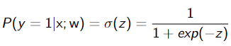
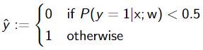
预测概率最高的类别

多分类逻辑回归，用softmax：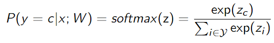

Gradient Descent 梯度下降：计算损失函数对整个训练集参数的梯度
Batch Gradient Descent 批量梯度下降：计算损失函数对小部分训练集参数的梯度
任何具有很多特征的模型都容易过度拟合其训练数据：训练准确率高，测试准确率低，用正则化解决：Lreg = L + αR(w)，α是正则化强度

还有典中典中典之正确率

统计语言模型

ngram：

Perplexity 测试集 x = [x1, …, xN ] 的逆概率，由词数 N 归一化：
衡量概率分布预测样本的好坏程度，通常是越低越好。
二元语言模型的困惑度有可能低于一元语言模型，是因为可以有更多上下文进行下一个词的预测。

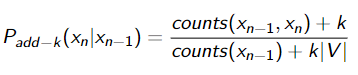
Smoothing平滑
Add-1（或拉普拉斯Laplace ）平滑对所有二元组的计数加一

衍生出来就是K平滑

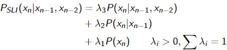
Interpolation

对于三元组语言模型，Interpolation操作是，计算一元组、二元组和三元组概率的加权平均值

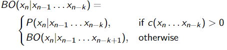
Backoff
从 k 的 n-gram 顺序开始，但如果计数为 0，则使用 k − 1

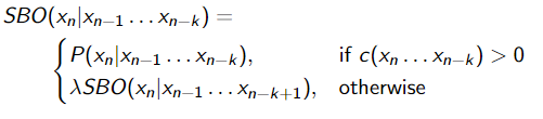
Absolute discounting

Stupid Backoff
经验之谈，λ = 0.4 效果很好

Extrinsic Evaluation

• Sentence completion
• Grammatical error correction: detecting “odd” sentences and propose alternatives 语法错误纠正
• Natural lanuage generation: prefer more “natural” sentences 自然语言生成
• Speech recognition 语音识别
• Machine translation 机器翻译

Intrinsic Evaluation

• Accuracy
• Perplexity
  -The lower the better
  -Can’t evaluate non probabilistic LMs

[自己想的
advantage: intrinsic evaluation is focus on maths formula and will not being influenced by other external factors
disadvantage : Intrinsic evaluation does not necessarily reflect the language model’s performance in real-world applications.
]

序列标注和词性标注POS tagging

• Part-of-Speech (POS) Tagging
  (x, y) = ([I , studied, in, X],
  [Pronoun, Verb, Preposition, ProperNoun])
• Named Entity Recognition
  (x, y) = ([Giannis, Antetokounmpo, plays, for , the, Bucks],
  [Person, Person, NotEnt, NotEnt, NotEnt, Org ])
• Machine Translation (reconstruct word alignments)
  (x, y) = ([la, maison, bleu],
  [the, house, blue])

数据由带有标签序列的单词序列组成：
Dtrain = {(x1, y1)…(xM , yM )}
xm = [x1, …xN ]
ym = [y1, …yN ]
学习预测最佳标签序列的模型 f：
y ∈ Y^N 是标签序列所有可能组合的集合，Y = {A, B, C …} 是每个词的可能类别。
用了markov模型，就用标签 y 替代单词
标签 yi（即 PoS 标签）是发出单词的隐藏状态
假设：POS 标签中的一阶马尔可夫（当前标签仅取决于先前标签），且每个单词仅取决于其 POS 标签
公式推导：

Maximum likelihood estimation 最大似然估计

一个例子：
高阶 HMM通常需要更长的上下文、更昂贵，收益通常很小。

逻辑回归也能提供序列标签的概率。
Conditional Random Field 条件随机场是给定一个词，当前词的候选标签和前一个词的标签，在每个时间步中使用（多类 LR）预测该词最可能的标签
分解每个句子 x = [x1, …xN ] 预测：
对每个单词Xn
构造CRF的特征向量例子：
φ1(xn, yn, yn−1, n) = 1， 如果 yn = ADVERB 并且第 n 个单词以“-ly”结尾；否则为 0。“usually”,”casually”
φ2(xn, yn, yn−1, n) = 1 ，如果 n = 1，yn = 动词，句子以问号结尾；否则为 0。“Is it true?”
CRF 通过最小化负对数似然目标进行训练：，也会使用随机梯度下降SGD

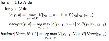
Viterbi

Viterbi score matrix标签集 Y，句子 x = [x1, …xN ]。对于带有标签 y 的单词 n，每个单元格包含最高概率。
一阶马尔可夫：只依赖于前一个标签 yn−1

Backpointer matrix：保留前一个标签而不是最高值，和Viterbi score matrix的区别是取argmax：

vertibi算法：
输入：词序列 x = [x1, …, xN ],概率 P(yn|xn, yn−1) ，让矩阵 = 1

beam search

Viterbi 通过评估所有选项执行精确搜索（在假设下），通过不精确来加快速度，即使用 Beam Search 避免标记一些候选序列。
beam search和vertibi总体一致，但在每一步只保留最好的 k 个假设。
如果beam size为1，则是贪婪算法。通常小于 10 的beam size接近精确搜索，但速度要快得多
从分支里选k个继续分支

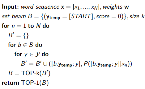
beam search 何时停止：假设产生 时，该假设算视为完成。通常停止状态设置为T个周期时长，或是N个完成的假设

Word2Vec

Forward Pass:

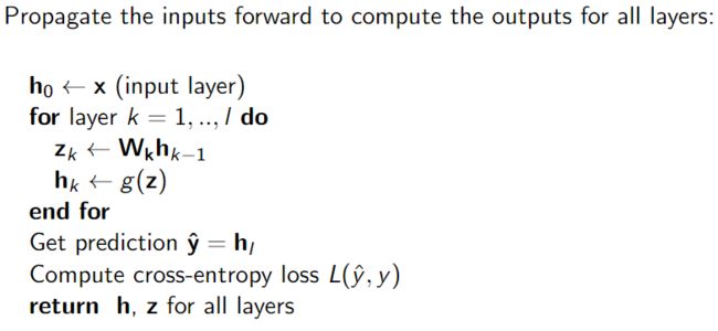
Backward Pass:

SGD：

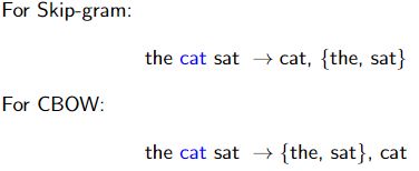
Skip-gram model 给定一个词预测它的上下文
Continuous BOW (CBOW) 给定上下文预测当前词

输入一个词，表示为词汇表上的one-hot向量
隐藏层，一个隐藏层大小为词汇量×隐藏大小（通常为300），线性激活函数
输出softmax 在词汇表上分别预测正确的词

Word2vec 结构：

Negative Sampling 更新正positive词的权重，加上少量（5-20​​）其他要输出0的词的权重
Subsampling frequent words 减少训练样本的数量

文本分类

方法 1：将 BOW 向量传递到一系列隐藏层中
方法 2：通过嵌入层传递one-hot向量以获得文档中每个词的嵌入，随后将其连接（或相加/平均）并传递到一系列隐藏层
方法二中通常嵌入层是预训练的（例如使用 Word2Vec）并且在训练期间不更新

信息提取

What is Information Extraction (IE)?
• a practically-motivated engineering discipline (models not necessarily inspired by nature)
• the extraction of structured information from unstructured (= textual) sources.
• its significance is connected to the growing amount of information in text and its potential use in systems (e.g. question answering)

IE tasks:

1 Named Entity Recognition 命名实体识别
• John Fitzgerald Kennedy, United States
2 Entity Disambiguation 实体消歧
• Jack is also known as John F Kennedy
3 Entity Coherence 实体一致性
• The word “He” makes reference to John F Kennedy
4 Relation Classification/Extraction 关系分类/提取
• The phrase “served as the 35th president” shows the relationship between John F Kennedy and United States
• Structured knowledge: (John F Kennedy, former president, United States)
5 Knowledge Base Population

Information Extraction System Architecture

• Text normalization: Reducing the text into a single canonical form
• Tokenization: Splitting the text into smaller units such as words or characters
• Stemming: Reducing inflectional form of words to their base form (e.g., eating, eats, eaten is reduced to eat)
• Lemmatization: similar to a stemming process but guided by a lexical knowledge base to obtain accurate word stems.
• POS tagger: Assigns part-of-speech tags to words in text
• Chunk parser: individual pieces of text and grouping them into meaningful grammatical chunks or syntactic units.
→ Feature Extraction/Learning: transforming text into numerical features
→ Named entity tagger: identify and classify entities
→ Relation Tagger: find relation between entities
→ Populate knowledge base with facts

Text Classification Example

• Feature extraction/engineering: using domain knowledge to extract features from data.
• Feature: a piece of evidence intended to help the classifier map the input to the right target class
• Feature vector: a vector −→ F , the components Fj = φj (dj ), of which are results applying a feature function to the data point dj .
• Example: “Spam vrs Ham” email?
number of “!” included in email body
length of the email in characters
occurrence of the word “cash” in the title or body.
• Example feature vectors:
(2, 2392, no) → HAM (genuine e-mail)
(4, 520, yes) → SPAM
(1, 2392, no) → HAM
(0, 16337, no) → HAM
(0, 61320, yes) → SPAM

Rule-based

• Human experts (computational linguists) write general linguistic rules and task-specific extraction rules.
• Example, trigger keywords, regular expressions and patterns.
• Rule-based rules are language dependent, suffer from human ingenuity, time consuming, difficult to adapt to changes.

Machine Learning based (supervised)

• Humans (domain experts) manually annotate text spans indicating entities, relations, facts, etc. in a training corpus;
• features are manually or automatically engineered (or a mixture of the two, e.g. using neural networks and dependency trees);
• these are used to extract information that statistically correlates with classes of entities,relations, etc.

Include:
• Hidden Markov Models (HMMs)
• Conditional Random Fields (CRF)
• Support Vector Machines (SVMs) and Softmax Function
• Artificial Neural Networks (NNs), in particular “deep” neural nets for sequence tagging (RNN, LSTM), CNN, GCN, BERT

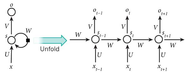
RNN

Recurrent Neural Networks (RNNs) to capture long-range dependencies in a document

选择上下文直到n-1
控制传播
包含所有单词的单词向量的矩阵，这里Xn选一个
Xn的概率分布：，这里V是权重矩阵

词向量 U，隐藏层和输出层参数 W，V
标准反向传播无法应用在RNN上，需要用Backpropagation Through Time：将图形展开 n 步并在更新中对梯度求和
RNN 无法捕获 long-range dependencies:
句子中的每个单词实际上只有一层，所有上下文信息都必须由隐藏层传递，且有梯度消失的情况。
梯度消失：最后一个单词的梯度通常永远不会到达第一个

RNN结构：
many to one: text classification
many to many (equal): PoS tagging
many to many (unequal): . machine translation, language generation, summarisation

Long-Short Term Memory (LSTM) network

LSTM在RNN基础上还使用了一个记忆单元来控制来自先前时间步长的哪些信息对预测有用
Forget gate : 从前面的步骤中丢弃什么信息
Input gate : 哪些新信息将存储在存储单元中
memory cell candidate values
用 input 和 output gates更新memory cell

Gated Recurrent Unit 是LSTM的变种
upgrade gate(结合 input and forget gates) :
Recurrent state （合并cell state与hidden state）:
output candidate values ：
output ：
encoder creates a representation of the source sentence
decoder uses that representation to generate the target sentence
RNN 学习单词和句子/文档表示
RNN 的训练速度比 Skip-Gram 慢，因此需要使用更少的数据
使用预训练词向量（例如 skipgram）来初始化 RNN 词向量
Bi-directional 双向 RNN 也可用于学习文档表示：一个 RNN 从头到尾解析输入，另一个从尾到头解析输入

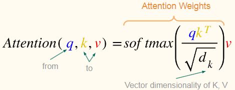
注意力机制

注意力机制：计算从 RNN 获得的所有上下文表示的线性加权和，将结果传递给输出层进行分类
再将c传递给输出层进行分类。
Attention 通常由相似度函数 φ 和 softmax 组成

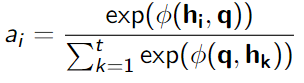
q 是一个可训练的向量（学习特定于任务的信息），
一些额外的操作：
用tanh：
缩放点积：

Input ：所有encoder隐藏状态 h1, …, hN；时间步 t 的decoder隐藏状态 St
Scores：score (st , hk ), k = 1…N
Weights：

Output：

Sequence to Sequence Model

例如：Machine Translation，Speech to Text，Image Captioning，Named entity recognition，Neural Music Generation

Neural Machine Translation (NMT) is Machine Translation using neural networks (as opposed to alignment and phrase based translation).
● Typically we use sequence-to-sequence models (seq2seq).
● These models are end-to-end differentiable

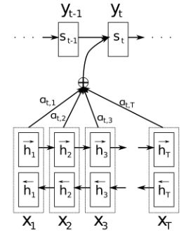
Self-Attention

Each vector receives a:
● Query (q): vector from which the attention is looking
● Key (k): vector at which the query looks to establish context
● Value (v): value of word being looked at, weighted based on context

Query旨在建立上下文，在这个例子中，单词“computer”（蓝色），通过Query 所有单词的每个Key来完成（黄色）
在这个例子里可能会将“science”确立为提供最多信息上下文的词。再通过 softmax 输出，并将每个value乘以与每个词相关的value（目标词）

Attention vs self-attention

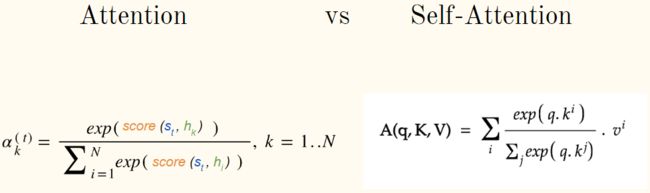
The query is similar to the current decoder step
(Query * Key) is similar to dot product scoring (where the key is equivalent to the encoder outputs
在将两者都推入 softmax 之后，我们将结果与自注意力中的值相乘，然后再对其求和
In RNN attention this is again the encoder states

Transfer Learning

Transfer learning: Re-use and adapt already pre-trained supervised machine learning models on a target task
：Different feature spaces in source and target domains, e.g. documents written in different languages (cross-lingual adaptation)
：Different marginal probability distributions in source and target domains, e.g. restaurant reviews vs electronic product reviews (domain adaptation)
：Different tasks (label sets), e.g. LM as source task and sentiment analysis as target task
：Different conditional probability distributions between source and target tasks, e.g. source and target documents are unbalanced regarding to their classes

BERT

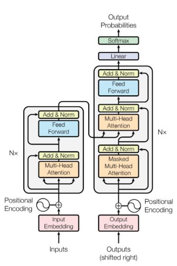
Encoder 12 layers: 2 sub-layers each
Sub-layer 1: Multi-head self-attention mechanism
Sub-layer 2: Position-wise fully connected layer
Output of each sublayer is combined with its input followed by layer norm
Input tokens are combined with a positional embedding (containing information for particular position in the sequence)

Adaptation

Initialise your encoder on the target task using the weights you learned in LM
Change the output layer of your network to match the target task
Freeze the weights of the pretrained word embeddings/encoder
Learn the weights of the output layer on the target task data
Unfreeze the weights of the pretrained components and fine-tune them (additional training steps with very small learning rate)
In ULMFiT, the LM encoder (LSTM) is fine-tuned on the target task data before adaptation