David Silver Lecture 8: Integrating Learning and Planning

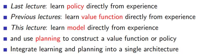
1 Introduction

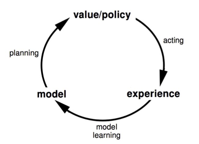
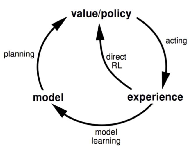
1.1 Model based Reinforcement Learning

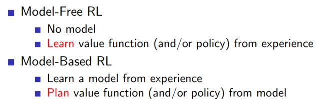
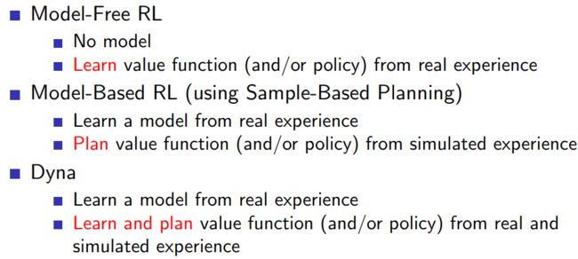
1.2 model based and model free RL

2 Model-Based Reinforcement Learning

2.1 outline

2.2 Learning a model

2.2.1 what is a model

model主要是指，state transitions和相应的reward。

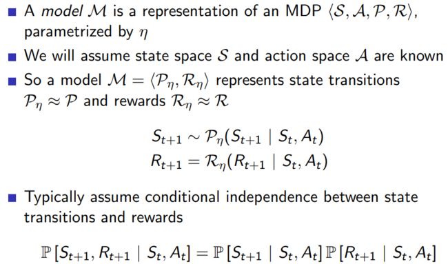
2.2.2 Model learning

2.2.3 Examples of Models

• table lookup model

import numpy as np

class TableModel:
    def __init__(self, num_states, num_actions):
        # Initialize the table with zeros
        self.table = np.zeros((num_states, num_actions, num_states))

    def update(self, state, action, next_state):
        # Increment the count for the observed transition
        self.table[state, action, next_state] += 1

    def predict(self, state, action):
        # Normalize the table to get probabilities
        prob = self.table[state, action] / np.sum(self.table[state, action])
        
        # Sample next state
        next_state = np.random.choice(np.arange(num_states), p=prob)
        
        return next_state

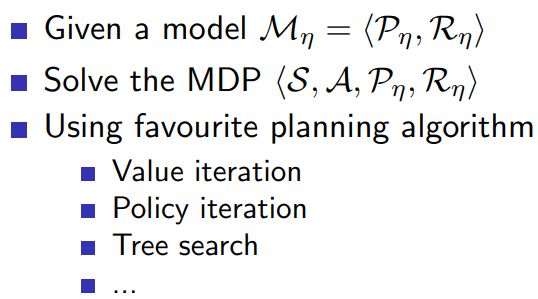
2.3 Planning with a model

2.3.1 Sample based planning

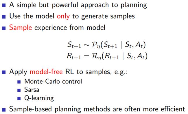
基于样本的规划(sample-based planning)方法是一种在模型中进行搜索的方法，以找到最优策略。这种方法的主要思想是通过模拟随机样本的方式来近似解决决策问题，而不是直接在整个状态空间上进行搜索。

一个简单的问题：假设我们有一个简单的迷宫问题。在每个时间步，代理可以选择上、下、左或右移动一步。我们的目标是找到从起始位置到目标位置的最短路径。

1.初始化 Q 值和 eligibility traces。
2.在给定的迷宫中，从起始位置开始，选择一个动作。初始动作可以是随机选择的，也可以是根据当前策略选择的。
3.执行选定的动作，观察结果状态和奖励。
4.在结果状态处，根据 SARSA(λ) 更新规则，选择下一个动作，并更新 Q 值和 eligibility traces。
5.重复步骤 3 和 4，直到到达目标状态或达到最大步数。
6.使用更新的 Q 值，更新策略。
7.通过模拟一系列随机样本，使用基于样本的规划方法更新策略。
8.重复步骤 2 到 7，直到策略收敛。

import numpy as np

# 迷宫的尺寸
size = (10, 10)
# 目标位置
goal = (9, 9)
# ε-贪心策略的参数
epsilon = 0.1
# 衰减因子
gamma = 0.95
# Sarsa(λ)的参数
lambda_ = 0.9
# 动作集合
actions = [(0, -1), (-1, 0), (0, 1), (1, 0)]
# 学习率
alpha = 0.5

# 初始化Q值和E痕迹
Q = np.zeros(size + (len(actions),))
E = np.zeros_like(Q)

# 对于每一步
for episode in range(1000):
    # 初始化状态
    state = (0, 0)
    # 选择一个动作
    if np.random.rand() < epsilon:
        action = np.random.choice(len(actions))
    else:
        action = np.argmax(Q[state])

    while state != goal:
        # 执行动作并观察结果
        next_state = (state[0] + actions[action][0], state[1] + actions[action][1])
        next_state = max(0, min(size[0]-1, next_state[0])), max(0, min(size[1]-1, next_state[1]))

        # 选择下一个动作
        if np.random.rand() < epsilon:
            next_action = np.random.choice(len(actions))
        else:
            next_action = np.argmax(Q[next_state])

        # 计算奖励
        reward = -1 if next_state != goal else 0

        # 更新Q值和E痕迹
        delta = reward + gamma * Q[next_state + (next_action,)] - Q[state + (action,)]
        E[state + (action,)] += 1
        Q += alpha * delta * E
        E *= gamma * lambda_

        # 移动到下一个状态
        state = next_state
        action = next_action

# 现在，Q值应该为每个状态动作对给出最优路径

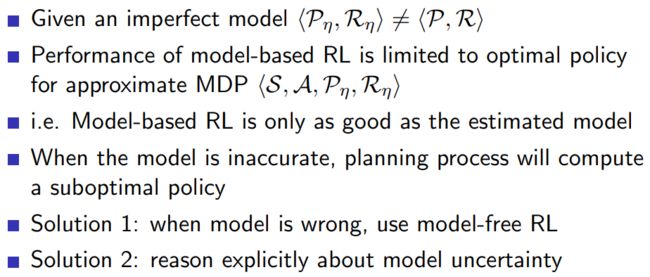
2.3.2 Planning with an Inaccurate Model

3 Integrated Architecture

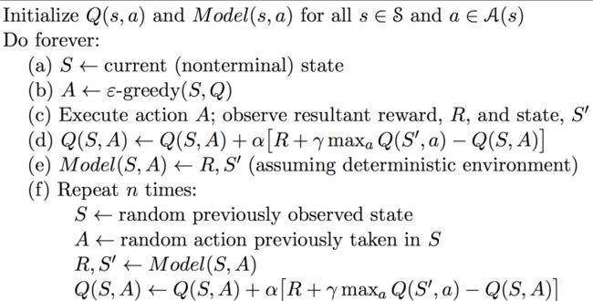
3.1 Dyna

在Dyna中，一个智能体同时进行两种类型的学习：直接从与环境的交互中学习（模型自由学习），以及通过模拟环境并从中学习（模型驱动学习）。Dyna架构的主要组件包括：

1智能体：智能体执行操作，观察结果，并进行学习。
2模型：模型预测结果，例如下一个状态和奖励。
3价值函数：价值函数（例如，Q函数）预测每个状态-动作对的价值。
4策略：策略决定智能体在每个状态下应执行的动作。

下面是Dyna架构的工作步骤：

1直接强化学习：智能体在环境中执行操作，观察结果，并直接从中更新价值函数。
2模型学习：智能体在环境中执行操作，观察结果，并从中学习模型。
3模型驱动学习：智能体使用模型进行模拟，并从模拟中更新价值函数。

Dyna架构的优点是，它能够同时利用模型自由和模型驱动的优点。模型自由学习可以直接从实际经验中学习，而模型驱动学习可以通过模拟来有效地利用已有知识。另一方面，Dyna架构的缺点是，它需要一个准确的模型才能有效。如果模型不准确，那么通过模型驱动学习产生的结果可能会误导智能体。

import numpy as np

# 参数设置
n_states = 5
n_actions = 2
n_steps = 1000
alpha = 0.1
gamma = 0.95
epsilon = 0.1
n_planning_steps = 5

# 初始化
Q = np.zeros((n_states, n_actions))
model = dict()

for step in range(n_steps):
    # 直接强化学习
    s = np.random.randint(n_states)
    a = np.random.choice([np.argmax(Q[s]), np.random.randint(n_actions)], p=[1-epsilon, epsilon])
    r = np.random.randn()
    s_ = np.random.randint(n_states)
    Q[s, a] += alpha * (r + gamma * np.max(Q[s_]) - Q[s, a])

    # 模型学习
    model[(s, a)] = (r, s_)

    # 模型驱动学习
    for _ in range(n_planning_steps):
        sa = list(model.keys())[np.random.randint(len(model))]
        r, s_ = model[sa]
        Q[sa] += alpha * (r + gamma * np.max(Q[s_]) - Q[sa])

print(Q)

算法步骤

4 Simulation Based Search

4.1 Outline

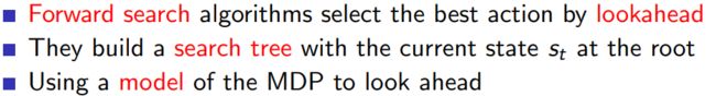
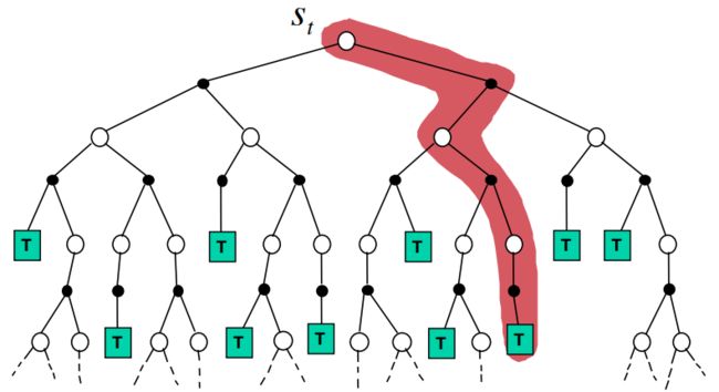
4.1.1 Forward search

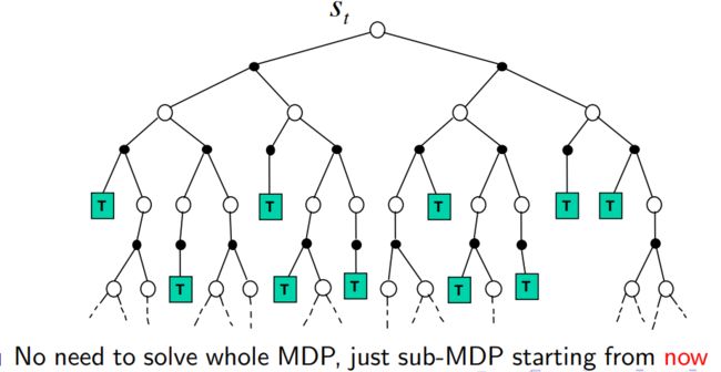
4.1.2 Simulation-based Search

模拟基础搜索（Simulation-Based Search）是一种强化学习方法，它利用模拟来预测智能体在环境中执行特定动作的结果，并据此选择最优的动作。这种方法通常用在环境模型已知或可学习的情况下。

• 优点：
  1减少了实际交互的需求：模拟基础搜索通过模拟环境来预测结果，而不需要实际在环境中执行动作，这大大减少了实际交互的需求。
  2提高了学习效率：由于模拟基础搜索可以在每次实际交互之间进行多次模拟，因此它可以更快地学习环境。

• 缺点
  1模型的准确性：模拟基础搜索的性能严重依赖于模型的准确性。如果模型不准确，那么模拟的结果可能会误导智能体。
  2计算成本：模拟基础搜索需要大量的计算资源来进行模拟，这可能会限制它在复杂环境中的应用。
  
  
  让我们考虑一个更为典型的强化学习问题，如MountainCar问题。在这个问题中，智能体需要驾驶一辆车从一个山谷中爬出来。车的引擎不够强，不能直接爬上山坡，因此必须利用动量来到达目标。

在这个问题中，我们可以使用模拟基础搜索来找到最佳的行动策略。我们的模型会模拟车在执行特定动作后的位置和速度，我们的策略将基于这些模拟结果来选择动作。这是一个典型的强化学习问题，因为智能体需要通过与环境的交互来学习如何最大化累积奖励。

在以下代码中，我们将使用OpenAI的gym库来设置MountainCar环境，并使用一种称为Monte Carlo Tree Search（MCTS）的模拟基础搜索算法来解决这个问题：

解决思路：
我们创建了一个名为Node的类，该类表示Monte Carlo Tree Search（MCTS）的一个节点。simulate函数负责执行模拟，它在每个步骤中选择一个动作，然后执行这个动作并添加新的子节点。我们的策略是一个简单的随机策略，它在每个步骤中随机选择一个动作。在每次模拟结束后，我们根据平均奖励选择最好的子节点作为下一步的状态。

import gym
import numpy as np

class Node:
    def __init__(self, state, parent=None):
        self.state = state
        self.parent = parent
        self.children = []
        self.rewards = []

    def add_child(self, child):
        self.children.append(child)

    def add_reward(self, reward):
        self.rewards.append(reward)

    def is_leaf(self):
        return len(self.children) == 0

    def is_root(self):
        return self.parent is None

    def get_average_reward(self):
        return np.mean(self.rewards)

def simulate(node, env, policy, max_steps=200):
    env.state = node.state
    for _ in range(max_steps):
        action = policy(env.state)
        state, reward, done, _ = env.step(action)
        child = Node(state, parent=node)
        node.add_child(child)
        node.add_reward(reward)
        node = child
        if done:
            break

def best_child(node):
    best_score = -np.inf
    best_child = None
    for child in node.children:
        score = child.get_average_reward()
        if score > best_score:
            best_score = score
            best_child = child
    return best_child

def mcts(state, env, policy, n_simulations=100):
    root = Node(state)
    for _ in range(n_simulations):
        simulate(root, env, policy)
    return best_child(root).state

env = gym.make('MountainCar-v0')

# Dummy policy
def policy(state):
    return env.action_space.sample()

# Initial state
state = env.reset()

# Run MCTS
for _ in range(200):
    next_state = mcts(state, env, policy)
    state = next_state
    env.render()

env.close()

4.2 Monte-Carlo Search

MCTS包括四个步骤：选择（Selection）、扩展（Expansion）、模拟（Simulation）和反向传播（Backpropagation）。在选择步骤，算法从根节点开始，按某种策略选择子节点，直到找到一个尚未完全扩展的节点。在扩展步骤，算法选择一个未被评估过的子节点进行扩展。在模拟步骤，算法模拟一次随机对战，得到此次对战的结果。在反向传播步骤，算法将模拟的结果反向传播到所有经过的节点，并更新这些节点的评估值。

Tic-Tac-Toe游戏

from copy import deepcopy
import numpy as np

class Node:
    def __init__(self, state, parent=None):
        self.state = state
        self.parent = parent
        self.children = []
        self.wins = 0
        self.visits = 0

    def add_child(self, child):
        self.children.append(child)

class TicTacToe:
    def __init__(self):
        self.board = np.zeros((3, 3))
        self.player = 1

    def get_valid_moves(self):
        return np.argwhere(self.board == 0)

    def make_move(self, move):
        self.board[move[0], move[1]] = self.player
        self.player = -1 if self.player == 1 else 1

    def game_over(self):
        for player in [-1, 1]:
            for axis in [0, 1]:
                if (self.board.sum(axis=axis) == player*3).any():
                    return True
            if np.diag(self.board).sum() == player*3 or np.diag(np.fliplr(self.board)).sum() == player*3:
                return True
        return False

    def get_winner(self):
        for player in [-1, 1]:
            for axis in [0, 1]:
                if (self.board.sum(axis=axis) == player*3).any():
                    return player
            if np.diag(self.board).sum() == player*3 or np.diag(np.fliplr(self.board)).sum() == player*3:
                return player
        return 0

def UCT(node):
    return node.wins / node.visits + np.sqrt(2*np.log(node.parent.visits)/node.visits)

def select(node):
    while len(node.children) > 0:
        node = max(node.children, key=UCT)
    return node

def expand(node, game):
    for move in game.get_valid_moves():
        game_copy = deepcopy(game)
        game_copy.make_move(move)
        node.add_child(Node(game_copy.board, parent=node))

def simulate(game):
    while not game.game_over():
        moves = game.get_valid_moves()
        move = moves[np.random.randint(len(moves))]
        game.make_move(move)
    return game.get_winner()

def backpropagate(node, result):
    while node is not None:
        node.visits += 1
        if result == 1:
            node.wins += 1
        node = node.parent

def mcts(game, n_simulations=100):
    root = Node(game.board)

    for _ in range(n_simulations):
        node = select(root)
        game_copy = deepcopy(game)
        game_copy.board = node.state
        if not game_copy.game_over():
            expand(node, game_copy)
            if len(node.children) > 0:
                node = node.children[np.random.randint(len(node.children))]
                game_copy.board = node.state
        result = simulate(game_copy)
        backpropagate(node, result)

    return max(root.children, key=lambda x: x.visits).state

game = TicTacToe()
while not game.game_over():
    print(game.board)
    if game.player == 1:
        moves = game.get_valid_moves()
        move = moves[np.random.randint(len(moves))]
    else:
        move = np.argwhere(mcts(game) != 0)[0]
    game.make_move(move)
print(game.board)

代码的实现思路
Node类：表示MCTS中的一个节点。每个节点都有一个状态（对应井字棋的棋盘），可能有一个父节点，有一系列的子节点，以及节点被访问的次数（visits）和在模拟游戏中赢得的次数（wins）。

TicTacToe类：表示井字棋游戏。棋盘被表示为一个3x3的矩阵，其中0表示空位，1表示玩家1的棋子，-1表示玩家2的棋子。游戏类包含了获取有效移动的方法（get_valid_moves），执行移动的方法（make_move），检查游戏是否结束的方法（game_over），和获取胜者的方法（get_winner）。

UCT函数：计算节点的上限置信区间（Upper Confidence Bound，UCT）。UCT用于在选择阶段决定哪个子节点应该被访问。它是一个基于节点的平均奖励和访问次数的值。

select函数：实现MCTS的选择阶段。从根节点开始，每次都选择UCT值最高的子节点，直到找到一个尚未完全扩展的节点。

expand函数：实现MCTS的扩展阶段。对于给定的节点和游戏状态，生成所有可能的下一步移动并添加为子节点。

simulate函数：实现MCTS的模拟阶段。对游戏进行随机模拟，直到游戏结束，然后返回游戏结果。

backpropagate函数：实现MCTS的反向传播阶段。更新从叶节点到根节点路径上的所有节点的访问次数和胜利次数。

mcts函数：实现MCTS算法的主循环。进行指定次数的模拟，然后返回访问次数最多的子节点的状态。

主循环：创建一个井字棋游戏，然后在游戏结束之前，轮流让玩家1（使用随机策略）和玩家2（使用MCTS）进行移动。

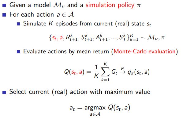
• simple Monte-carlo search
  根据现有的规则，对所有的action，simulate k 步，更新Q值，选择最好的action
  

• Monte-Carlo Tree Search Evaluation
  
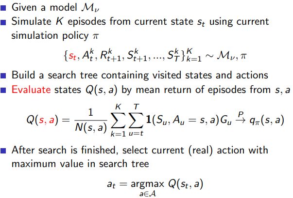
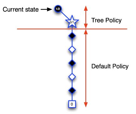
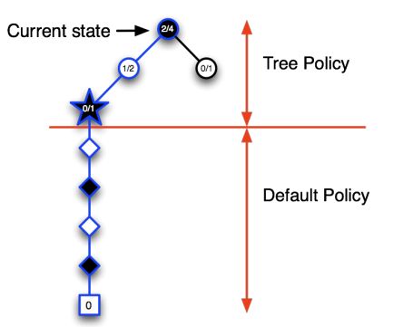
  在MCTS中，找到最好的动作主要涉及以下四个步骤：

• 选择(Selection)：从根节点开始，按照某种策略（如 UCB1）选择子节点，直到找到一个未完全扩展或终止的节点。

• 扩展(Expansion)：如果找到的节点不是终止节点，那么就创建一个或多个新的子节点，并选择其中一个。

• 模拟(Simulation)：从选定的节点开始，进行 Monte Carlo 模拟，即按照一定策略（通常是随机策略）选择动作，直到游戏结束。

• 回传(Backpropagation)：根据模拟的结果，更新从根节点到选定节点路径上的所有节点。通常，每个节点会记录模拟的次数和获得的总奖励。

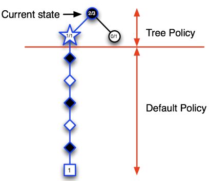
通过反复执行这四个步骤，MCTS会逐渐扩展其游戏树，并越来越偏向于选择有希望的动作。最后，从根节点开始，选择模拟次数最多或平均奖励最高的动作，就是 MCTS 找到的最好动作。

这个过程的一个关键点是，MCTS 利用了游戏树和回传步骤来维护关于每个状态和动作的信息，这使得 MCTS 能够根据以前的模拟结果来指导未来的模拟。这一点是简单的 Monte Carlo 搜索所没有的，它会独立地对每个动作进行模拟，而忽略了这些动作之间可能的关系。

4.3 MCTS in Go

• position Evaluation in Go
  
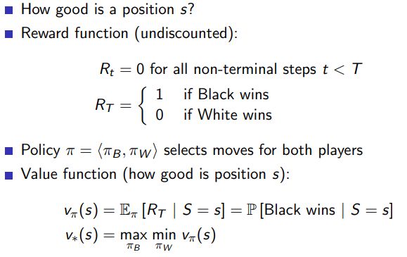
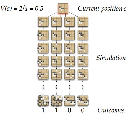
• Monte-carlo Evaluation in Go
  
• Applying Monte-Carlo Tree Search
  
  
  
  
  
• Advantages of MC Tree Search
  

4.4 Temporal Difference Search

• Dyna-2