《视觉SLAM十四讲》手写高斯牛顿—笔记记录

《视觉SLAM十四讲》手写高斯牛顿—笔记记录

我们的最终目的：使用高斯牛顿法，拟合参数abc
我们的实际小目标：求解增量方程得到ΔX（有了Δx就可以不停的迭代Eabc使得拟合Rabc啦）

三个步骤：
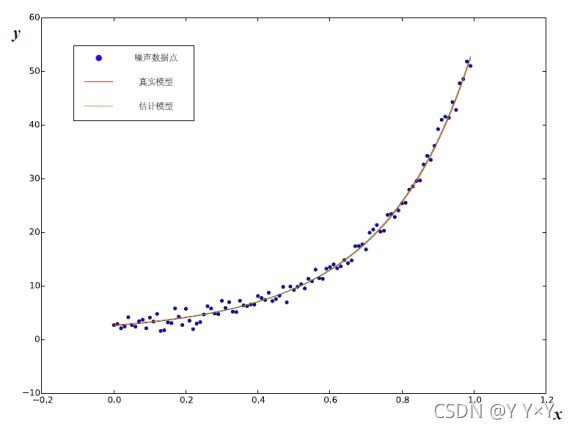
1、先根据模型生成x，y的真值，并在真值中添加高斯分布的噪声
2、使用高斯牛顿法进行迭代
3、求解高斯牛顿法的增量方程

首先定义真实的a，b，c参数值为ar，br，cr
	这三个也是我们要拟合的最终目标，最终的拟合结果跟这三个值越接近越好

double ar = 1.0, br = 2.0, cr = 1.0;

然后定义初始的估计参数值ae，be，ce
	这三个就是用于迭代的，最后效果最好是ae，be，ce迭代到与ar，br，cr一样。

 double ae = 2.0, be = -1.0, ce = 5.0; 

然后我们假设有100个数据点，设置噪声值sigma

第一步，根据模型生成X，Y的真值，并添加高斯分布的噪声

  vector<double> x_data, y_data;      // 数据
  for (int i = 0; i < N; i++) {
    double x = i / 100.0;
    x_data.push_back(x);
    y_data.push_back(exp(ar * x * x + br * x + cr) + rng.gaussian(w_sigma * w_sigma));
  }

第二步，使用高斯牛顿法进行迭代
迭代次数设为100次
定义误差：

     double error = yi - exp(ae * xi * xi + be * xi + ce);

然后分别对每个误差项对a，b，c进行求导，然后生成雅可比矩阵

      Vector3d J; // 雅可比矩阵
      J[0] = -xi * xi * exp(ae * xi * xi + be * xi + ce);  // de/da
      J[1] = -xi * exp(ae * xi * xi + be * xi + ce);  // de/db
      J[2] = -exp(ae * xi * xi + be * xi + ce);  // de/dc

然后求解海塞矩阵H和偏移量b

     H += inv_sigma * inv_sigma * J * J.transpose();
      b += -inv_sigma * inv_sigma * error * J;

第三步，求解高斯牛顿法的增量方程（相当于梯度下降的Δx，就是向前迈一小步~）
这里的关键语句是Vector3d dx = H.ldlt().solve(b);
涉及一个eigen库中的LDLT分解，其中L为一下三角形单位矩阵（即主对角线元素皆为1），D为一对角矩阵（只在主对角线上有元素，其余皆为零），L^T为L的转置矩阵。

    // 求解线性方程 Hx=b
    Vector3d dx = H.ldlt().solve(b);
    if (isnan(dx[0])) {
      cout << "result is nan!" << endl;
      break;
    }

    if (iter > 0 && cost >= lastCost) {
      cout << "cost: " << cost << ">= last cost: " << lastCost << ", break." << endl;
      break;
    }

    ae += dx[0];
    be += dx[1];
    ce += dx[2];
    
    lastCost = cost;   //更新损失

完整代码如下：

#include 
#include 
#include 
#include 
#include 

using namespace std;
using namespace Eigen;

//先根据模型生成x，y的真值
//在真值中添加高斯分布的噪声
//使用高斯牛顿法从带噪声的数据拟合参数模型

int main(int argc, char **argv) {
  double ar = 1.0, br = 2.0, cr = 1.0;         // 真实参数值  最后就是要迭代到跟这个真值接近
  double ae = 2.0, be = -1.0, ce = 5.0;        // 估计参数值  随便给定的一个初值，用于迭代到真值附近
  int N = 100;                                 // 数据点
  double w_sigma = 1.0;                        // 噪声Sigma值
  double inv_sigma = 1.0 / w_sigma;
  cv::RNG rng;                                 // OpenCV随机数产生器

  vector<double> x_data, y_data;      // 数据
  for (int i = 0; i < N; i++) {
    double x = i / 100.0;
    x_data.push_back(x);
    y_data.push_back(exp(ar * x * x + br * x + cr) + rng.gaussian(w_sigma * w_sigma));
  }

  // 开始Gauss-Newton迭代
  int iterations = 100;    // 迭代次数
  double cost = 0, lastCost = 0;  // 本次迭代的cost和上一次迭代的cost

  chrono::steady_clock::time_point t1 = chrono::steady_clock::now();
  for (int iter = 0; iter < iterations; iter++)
  {
    Matrix3d H = Matrix3d::Zero();             // Hessian = J^T W^{-1} J in Gauss-Newton
    Vector3d b = Vector3d::Zero();             // bias
    cost = 0;

    for (int i = 0; i < N; i++) {
      double xi = x_data[i], yi = y_data[i];  // 第i个数据点
      double error = yi - exp(ae * xi * xi + be * xi + ce);
      Vector3d J; // 雅可比矩阵
      J[0] = -xi * xi * exp(ae * xi * xi + be * xi + ce);  // de/da
      J[1] = -xi * exp(ae * xi * xi + be * xi + ce);  // de/db
      J[2] = -exp(ae * xi * xi + be * xi + ce);  // de/dc

      H += inv_sigma * inv_sigma * J * J.transpose();
      b += -inv_sigma * inv_sigma * error * J;

      cost += error * error;
    }

    // 求解线性方程 Hx=b
    Vector3d dx = H.ldlt().solve(b);
    if (isnan(dx[0])) {
      cout << "result is nan!" << endl;
      break;
    }

    if (iter > 0 && cost >= lastCost) {
      cout << "cost: " << cost << ">= last cost: " << lastCost << ", break." << endl;
      break;
    }

    ae += dx[0];
    be += dx[1];
    ce += dx[2];

    lastCost = cost;

    cout << "total cost: " << cost << ", \t\tupdate: " << dx.transpose() <<
         "\t\testimated params: " << ae << "," << be << "," << ce << endl;
  }

  chrono::steady_clock::time_point t2 = chrono::steady_clock::now();
  chrono::duration<double> time_used = chrono::duration_cast<chrono::duration<double>>(t2 - t1);
  cout << "solve time cost = " << time_used.count() << " seconds. " << endl;

  cout << "estimated abc = " << ae << ", " << be << ", " << ce << endl;
  return 0;
}

最终结果：

/home/yjc/SLAM_Study/ch6/cmake-build-debug/gaussNewton
total cost: 3.19575e+06, 		update: 0.0455771  0.078164 -0.985329		estimated params: 2.04558,-0.921836,4.01467
total cost: 376785, 		update:  0.065762  0.224972 -0.962521		estimated params: 2.11134,-0.696864,3.05215
total cost: 35673.6, 		update: -0.0670241   0.617616  -0.907497		estimated params: 2.04432,-0.0792484,2.14465
total cost: 2195.01, 		update: -0.522767   1.19192 -0.756452		estimated params: 1.52155,1.11267,1.3882
total cost: 174.853, 		update: -0.537502  0.909933 -0.386395		estimated params: 0.984045,2.0226,1.00181
total cost: 102.78, 		update: -0.0919666   0.147331 -0.0573675		estimated params: 0.892079,2.16994,0.944438
total cost: 101.937, 		update: -0.00117081  0.00196749 -0.00081055		estimated params: 0.890908,2.1719,0.943628
total cost: 101.937, 		update:   3.4312e-06 -4.28555e-06  1.08348e-06		estimated params: 0.890912,2.1719,0.943629
total cost: 101.937, 		update: -2.01204e-08  2.68928e-08 -7.86602e-09		estimated params: 0.890912,2.1719,0.943629
cost: 101.937>= last cost: 101.937, break.
solve time cost = 0.000237057 seconds. 
estimated abc = 0.890912, 2.1719, 0.943629

进程已结束，退出代码为 0