从简单线性回归到TensorFlow深度学习

大家好，人工智能近年来变得越来越流行，学习人工智能的需求也随之增加，尤其是许多IT专业人士希望利用机器学习的强大功能，但面临不小的挑战，尤其是在理论和数学上。

步骤1：线性回归

线性回归是一种统计学中常用的回归分析方法，用于建立一个自变量和一个或多个因变量之间的关系模型。在线性回归中，我们假设自变量和因变量之间存在一个线性关系，即因变量的值可以通过对自变量进行线性组合来预测。

线性回归可以用于解决各种问题，例如根据房屋面积、卧室数量、地理位置等因素来预测房价，或者根据广告投入、用户点击率等因素来预测销售额等。

在线性回归中，我们通常使用最小二乘法来估计模型参数，即通过最小化预测值与实际值之间的差异来确定自变量的系数。线性回归还可以通过引入多项式项、交互项等来建立更复杂的模型，以更好地适应实际情况。

下图通过随机生成一些数据，并进行了可视化：

import numpy as np
import matplotlib.pyplot as plt
from helpers import generate_data_lin, plot_linear_model, plot_loss_history

X, y = generate_data_lin(samples=100)
plot_data(X, y)

 将初始斜率和截距设为0：

# 初始化模型系数
slope = 0
bias  = 0

# 绘制未经训练的模型
plot_linear_model(X, y, slope, bias)

 实现损失函数、计算模型系数的梯度：

learning_rate = 0.01
epochs = 100
loss_history = []

# TODO: 实现损失函数(MSE)
def loss(X, y, slope, bias):
    return 0

# TODO: 计算模型系数的梯度
def gradient(X, y, slope, bias):
    return 0, 0

for i in range(epochs):    
    # 计算梯度
    slope_g, bias_g = gradient(X, y, slope, bias)
        
    # 更新系数
    slope -= slope_g * learning_rate
    bias  -= bias_g  * learning_rate
    
    # 更新损失历史
    loss_history.append(loss(X, y, slope, bias))
    
plot_linear_model(X, y, slope, bias)
plot_loss_history(loss_history)

在这个例子中使用的超参数不多，使用少量的超参数（学习率和周期数）有助于更好地理解它们在训练过程中的作用。

步骤2：多项式回归

从线性回归开始，多项式回归将说明如何添加其他非线性特征（有效地增加模型的复杂性），使我们能够建模更复杂的数据。

由于最终目标是实现神经网络，固定系数的数量可以降低抽象级别。这就是为什么我们通常会使用三次多项式的原因：

import numpy as np
import matplotlib.pyplot as plt
from helpers import generate_data_poly, plot_poly_model, plot_loss_history

X_train, y_train, X_test, y_test = generate_data_poly(samples=100, test_ratio=0.2)
plot_data(X_train, y_train, X_test, y_test)

 

# 用任意的值初始化模型系数
model_coefs = np.array([0, 0.1, 0.1, -0.1])

# 绘制未经训练的模型
plot_poly_model(X_train, y_train, model_coefs)

 和之前一样，实现损失函数(MSE)并计算模型系数的梯度：

learning_rate = 0.01
epochs = 100
train_loss_history = []
test_loss_history = []

# TODO: 实现损失函数(MSE)
def loss(X, y, model_coefs):
    return 0

# TODO: 计算模型系数的梯度
def gradient(X, y, coef):
    d0 = 0
    d1 = 0
    d2 = 0
    d3 = 0
    return np.array([d0, d1, d2, d3])

for i in range(epochs):    
    # 计算梯度
    coefs_g = gradient(X, y, model_coefs)
        
    # 更新系数
    model_coefs -= codefs_g * learning_rate
    
    # 更新损失历史
    train_loss_history.append(loss(X_train, y_train, model_coefs))
    test_loss_history.append(loss(X_test, y_test, model_coefs))
    
plot_poly_model(X_test, y_test, model_coefs)
plot_loss_history(train_loss_history, test_loss_history)

步骤3：神经网络回归

最后，我们可以基于简单线性回归和多项式回归，从计算图的角度来处理神经网络，可以将神经网络看作手动计算特征的模型。

从三次多项式（四个系数）到具有四个神经元的神经网络的转变非常无缝。这种比较是神经网络可以被视为对任意数量的计算单元（神经元）的抽象的绝佳说明。尽管每个神经元的单独能力较弱，但在数量较大时它们变得非常强大，因为它们使我们能够统一地计算梯度，从而显著地简化了训练过程。

使用TensorFlow创建神经网络模型：

import matplotlib.pyplot as plt
import numpy as np
from tensorflow.keras.models import Sequential
from tensorflow.keras.layers import Dense, Input
from helpers import generate_data_poly, plot_nn_model

X_train, y_train, X_test, y_test = generate_data_poly(samples=100, test_ratio=0.2)

model = Sequential([
    Input(1),
    Dense(4, activation='relu'),
    Dense(1)
])

model.compile(loss='mse')

model.fit(
    X_train,
    y_train,
    epochs=50,
    validation_data=[X_test, y_test],
    verbose=0
)

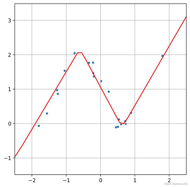
plot_nn_model(X_test, y_test, model)

 修改模型，使用Dense(32, activation='relu')：

model = Sequential([
    Input(1),
    Dense(32, activation='relu'),
    Dense(1)
])

model.compile(loss='mse')

model.fit(
    X_train,
    y_train,
    epochs=300,
    validation_data=[X_test, y_test],
    verbose=0
)

plot_nn_model(X_test, y_test, model)

 修改模型，再添加一个Dense(16, activation='relu')：

model = Sequential([
    Input(1),
    Dense(32, activation='relu'),
    Dense(16, activation='relu'),
    Dense(1)
])

model.compile(loss='mse')

model.fit(
    X_train,
    y_train,
    epochs=300,
    validation_data=[X_test, y_test],
    verbose=0
)

plot_nn_model(X_test, y_test, model)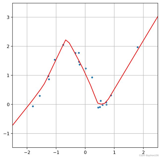

 

综上所述，在机器学习和统计学中，模型参数是指用来描述模型的一组数值或向量。这些参数可以被调整或优化，以使模型能够更好地拟合训练数据，从而提高模型的预测性能。

模型参数的意义通常取决于具体的模型类型。例如，在线性回归中，模型参数包括自变量的系数和截距项，它们描述了自变量和因变量之间的线性关系。在神经网络中，模型参数包括每个神经元的权重和偏置项，它们描述了神经元之间的连接方式和激活规律。