matlab使用教程(26)—常微分方程的求解
1.求解非刚性 ODE
本页包含两个使用 ode45 来求解非刚性常微分方程的示例。MATLAB® 提供几个非刚性 ODE 求解器。
• ode45
• ode23
• ode78
• ode89
• ode113
对于大多数非刚性问题,ode45 的性能最佳。但对于允许较宽松的误差容限或刚度适中的问题,建议使用ode23 。同样,对于具有更严格误差容限的问题,或当计算 ODE 函数的计算成本很高时, ode113 可能比ode45 更高效。 ode78 和 ode89 是高阶求解器,在精度对稳定性至关重要的长时积分中表现出色。
如果非刚性求解器需要很长时间才能解算问题或总是无法完成积分,则该问题可能是刚性问题。
2.1 示例:非刚性 van der Pol 方程
van der Pol 方程为二阶 ODE

ODE 方程组必须编码为 ODE 求解器能够使用的函数文件。ODE 函数的一般函数形式为
dydt = odefun(t,y) 即,函数必须同时接受 t 和 y 作为输入,即使它没有将 t 用于任何计算时亦如此。
![]()
function dydt = vdp1(t,y)
%VDP1 Evaluate the van der Pol ODEs for mu = 1
%
% See also ODE113, ODE23, ODE45.
% Jacek Kierzenka and Lawrence F. Shampine
% Copyright 1984-2014 The MathWorks, Inc.
dydt = [y(2); (1-y(1)^2)*y(2)-y(1)];
使用 ode45 函数、时间区间 [0 20] 和初始值 [2 0] 来解算该 ODE。输出为时间点列向量 t 和解数组 y 。 y 中的每一行都与 t 的相应行中返回的时间相对应。 y 的第一列与y1相对应,第二列与y2相对应。
[t,y] = ode45(@vdp1,[0 20],[2; 0]); 绘制y1和y2的解对 t 的图。
plot(t,y(:,1),'-o',t,y(:,2),'-o')
title('Solution of van der Pol Equation (\mu = 1) using ODE45');
xlabel('Time t');
ylabel('Solution y');
legend('y_1','y_2')
vdpode 函数可求解同一问题,但它接受的是用户指定的μ值。随着μ的增大,van der Pol 方程组将变成刚性。例如,对于值μ=1000,您需要使用 ode15s 等刚性求解器来求解该方程组。
2.2 示例:非刚性欧拉方程
对于专用于非刚性问题的 ODE 求解器,不受外力作用的刚体对应的欧拉方程是其标准测试问题。这些方程包括

函数文件 rigidode 定义此一阶方程组,并在时间区间 [0 12] 上使用初始条件向量 [0; 1; 1](该向量对应于y1、y2和y3的初始值)对该方程组进行求解。局部函数 f(t,y) 用于编写该方程组的代码。
rigidode 在调用 ode45 时未使用任何输出参数,因此求解器会在每一步之后使用默认的输出函数odeplot 自动绘制解点。
function rigidode
%RIGIDODE Euler equations of a rigid body without external forces.
% A standard test problem for non-stiff solvers proposed by Krogh. The
% analytical solutions are Jacobian elliptic functions, accessible in
% MATLAB. The interval here is about 1.5 periods; it is that for which
% solutions are plotted on p. 243 of Shampine and Gordon.
%
% L. F. Shampine and M. K. Gordon, Computer Solution of Ordinary
% Differential Equations, W.H. Freeman & Co., 1975.
%
% See also ODE45, ODE23, ODE113, FUNCTION_HANDLE.
% Mark W. Reichelt and Lawrence F. Shampine, 3-23-94, 4-19-94
% Copyright 1984-2014 The MathWorks, Inc.
tspan = [0 12];
y0 = [0; 1; 1];
% solve the problem using ODE45
figure;
ode45(@f,tspan,y0);
% --------------------------------------------------------------------------
function dydt = f(t,y)
dydt = [ y(2)*y(3)
 -y(1)*y(3)
 -0.51*y(1)*y(2) ];
通过调用 rigidode 函数来解算非刚性欧拉方程。
rigidode
title('Solution of Rigid Body w/o External Forces using ODE45')
legend('y_1','y_2','y_3','Location','Best')
2.求解刚性 ODE
本页包含两个使用 ode15s 解算刚性常微分方程的示例。MATLAB® 拥有四个专用于刚性 ODE 的求解器。
• ode15s
• ode23s
• ode23t
• ode23tb
对于大多数刚性问题,ode15s 的性能最佳。但如果问题允许较宽松的误差容限,则 ode23s 、 ode23t 和ode23tb 可能更加高效。
2.1 什么是刚性 ODE?
对于一些 ODE 问题,求解器采用的步长被强制缩小为与积分区间相比过小的级别,甚至在解曲线平滑的区域亦如此。这些步长可能过小,以至于遍历很短的时间区间都可能需要数百万次计算。这可能导致求解器积分失败,即使积分成功也需要花费很长时间。
导致 ODE 求解器出现此行为的方程称为刚性方程。刚性 ODE 造成的问题是,显式求解器(例如 ode45)获取解的速度慢得令人无法忍受。这是将 ode45 与 ode23 、 ode78 、 ode89 和 ode113 一同归类为非刚性求解器的原因所在。
专用于刚性 ODE 的求解器称为刚性求解器,它们通常在每一步中完成更多的计算工作。这样做的好处是,它们能够采用大得多的步长,并且与非刚性求解器相比提高了数值稳定性。
2.2 求解器选项
对于刚性问题,使用 odeset 指定 Jacobian 矩阵尤为重要。刚性求解器使用 Jacobian 矩阵
来预测 ODE 在积分过程中的局部行为,因此提供 Jacobian 矩阵(或者对于大型稀疏方程组提供其稀疏模式)对于提高效率和可靠性而言至关重要。使用 odeset 的 Jacobian 、 JPattern 或 Vectorized 选项来指定 Jacobian 的相关信息。如果没有提供 Jacobian,则求解器将使用有限差分对其进行数值预测。有关其他求解器选项的完整列表,请参阅 odeset 。
2.3 示例:刚性 van der Pol 方程
van der Pol 方程为二阶 ODE

其中μ>0为标量参数。当μ=1时,生成的 ODE 方程组为非刚性方程组,可以使用 ode45 轻松求解。但如果将μ增大至 1000,则解会发生显著变化,并会在明显更长的时间段中显示振荡。求初始值问题的近似解变得更加复杂。由于此特定问题是刚性问题,因此专用于非刚性问题的求解器(如 ode45)的效率非常低下且不切实际。针对此问题应改用 ode15s 等刚性求解器。
通过执行代换,将该 van der Pol 方程重写为一阶 ODE 方程组。生成的一阶 ODE 方程组为

vdp1000 函数使用μ=1000计算 van der Pol 方程。
function dydt = vdp1000(t,y)
%VDP1000 Evaluate the van der Pol ODEs for mu = 1000.
%
% See also ODE15S, ODE23S, ODE23T, ODE23TB.
% Jacek Kierzenka and Lawrence F. Shampine
% Copyright 1984-2014 The MathWorks, Inc.
dydt = [y(2); 1000*(1-y(1)^2)*y(2)-y(1)];
使用 ode15s 函数和初始条件向量 [2; 0] ,在时间区间 [0 3000] 上解算此问题。由于是标量,因此仅绘制解的第一个分量。
[t,y] = ode15s(@vdp1000,[0 3000],[2; 0]);
plot(t,y(:,1),'-o');
title('Solution of van der Pol Equation, \mu = 1000');
xlabel('Time t');
ylabel('Solution y_1');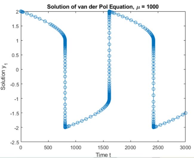
vdpode 函数也可以求解同一问题,但它接受的是用户指定的μ值。随着μ的增大,该方程组的刚性逐渐增强。
2.4 示例:稀疏 Brusselator 方程组
经典 Brusselator 方程组可能为大型刚性稀疏矩阵。Brusselator 方程组可模拟化学反应中的扩算,并表示为涉及u、v、u' 和v'的方程组。

函数文件 brussode 使用α=1/50在时间区间 [0,10] 上对这组方程进行求解。初始条件为

函数调用 brussode(N)(其中N≥2)为方程组中的 N(对应于网格点数量)指定值。默认情况下,brussode 使用N=20。
brussode 包含一些子函数:
• 嵌套函数 f(t,y) 用于编写 Brusselator 问题的方程组代码,并返回一个向量。
• 局部函数 jpattern(N) 返回由 1 和 0 组成的稀疏矩阵,从而显示 Jacobian 矩阵中非零值的位置。此矩阵将赋给 options 结构体的 JPattern 字段。ODE 求解器使用此稀疏模式,生成稀疏矩阵形式的Jacobian 数值矩阵。在问题中提供此稀疏模式可将生成 2N×2N Jacobian 矩阵所需的函数计算量从2N 次大幅减少至仅仅 4 次。
function brussode(N)
%BRUSSODE Stiff problem modelling a chemical reaction (the Brusselator).
% The parameter N >= 2 is used to specify the number of grid points; the
% resulting system consists of 2N equations. By default, N is 20. The
% problem becomes increasingly stiff and increasingly sparse as N is
% increased. The Jacobian for this problem is a sparse constant matrix
% (banded with bandwidth 5).
%
% The property 'JPattern' is used to provide the solver with a sparse
% matrix of 1's and 0's showing the locations of nonzeros in the Jacobian
% df/dy. By default, the stiff solvers of the ODE Suite generate Jacobians
% numerically as full matrices. However, when a sparsity pattern is
% provided, the solver uses it to generate the Jacobian numerically as a
% sparse matrix. Providing a sparsity pattern can significantly reduce the
% number of function evaluations required to generate the Jacobian and can
% accelerate integration. For the BRUSSODE problem, only 4 evaluations of
% the function are needed to compute the 2N x 2N Jacobian matrix.
%
% Setting the 'Vectorized' property indicates the function f is
% vectorized.
%
% E. Hairer and G. Wanner, Solving Ordinary Differential Equations II,
% Stiff and Differential-Algebraic Problems, Springer-Verlag, Berlin,
% 1991, pp. 5-8.
%
% See also ODE15S, ODE23S, ODE23T, ODE23TB, ODESET, FUNCTION_HANDLE.
% Mark W. Reichelt and Lawrence F. Shampine, 8-30-94
% Copyright 1984-2014 The MathWorks, Inc.
% Problem parameter, shared with the nested function.
if nargin<1
N = 20;
end
tspan = [0; 10];
y0 = [1+sin((2*pi/(N+1))*(1:N)); repmat(3,1,N)];
options = odeset('Vectorized','on','JPattern',jpattern(N));
[t,y] = ode15s(@f,tspan,y0,options);
u = y(:,1:2:end);
x = (1:N)/(N+1);
figure;
surf(x,t,u);
view(-40,30);
xlabel('space');
ylabel('time');
zlabel('solution u');
title(['The Brusselator for N = ' num2str(N)]);
% -------------------------------------------------------------------------
% Nested function -- N is provided by the outer function.
%
function dydt = f(t,y)
% Derivative function
c = 0.02 * (N+1)^2;
dydt = zeros(2*N,size(y,2)); % preallocate dy/dt

% Evaluate the 2 components of the function at one edge of the grid
% (with edge conditions).
i = 1;
dydt(i,:) = 1 + y(i+1,:).*y(i,:).^2 - 4*y(i,:) + c*(1-2*y(i,:)+y(i+2,:));
dydt(i+1,:) = 3*y(i,:) - y(i+1,:).*y(i,:).^2 + c*(3-2*y(i+1,:)+y(i+3,:));

% Evaluate the 2 components of the function at all interior grid points.
i = 3:2:2*N-3;
dydt(i,:) = 1 + y(i+1,:).*y(i,:).^2 - 4*y(i,:) + ...
c*(y(i-2,:)-2*y(i,:)+y(i+2,:));
dydt(i+1,:) = 3*y(i,:) - y(i+1,:).*y(i,:).^2 + ...
c*(y(i-1,:)-2*y(i+1,:)+y(i+3,:));

% Evaluate the 2 components of the function at the other edge of the grid
% (with edge conditions).
i = 2*N-1;
dydt(i,:) = 1 + y(i+1,:).*y(i,:).^2 - 4*y(i,:) + c*(y(i-2,:)-2*y(i,:)+1);
dydt(i+1,:) = 3*y(i,:) - y(i+1,:).*y(i,:).^2 + c*(y(i-1,:)-2*y(i+1,:)+3);
end
% -------------------------------------------------------------------------
end % brussode


% ---------------------------------------------------------------------------
% Subfunction -- the sparsity pattern
%
function S = jpattern(N)
% Jacobian sparsity pattern
B = ones(2*N,5);
B(2:2:2*N,2) = zeros(N,1);
B(1:2:2*N-1,4) = zeros(N,1);
S = spdiags(B,-2:2,2*N,2*N);
end
% ---------------------------------------------------------------------------
通过运行函数 brussode,对N=20时的 Brusselator 方程组求解。
brussode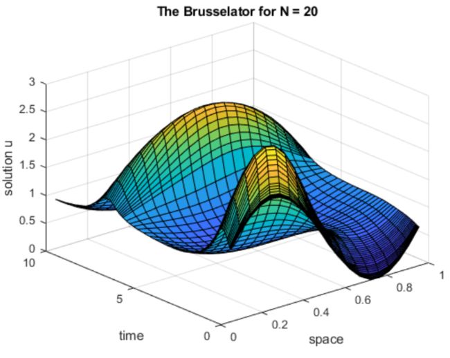
通过为 brussode 指定输入,对N=50时的方程组求解。
brussode(50)