python求遍历、最短路径、最小生成树、旅行商问题并绘图展示

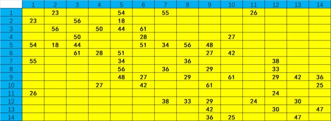
一、源数据

二、python程序

(1) 数据预处理

import numpy as np
import pandas as pd
from scipy.sparse import coo_matrix
import networkx as nx
import matplotlib.pyplot as plt

# 避免图片无法显示中文
plt.rcParams['font.sans-serif']=['SimHei']
# 显示所有列
pd.set_option('display.max_columns', None)
pd.set_option('display.width', 1000)

# 读取数据
data=pd.read_excel('data.xlsx',sheet_name='Sheet1',index_col=0)
data=data.fillna(0)
print('矩阵的空值以0填充：\n',data)
coo=coo_matrix(np.array(data))
# 矩阵行列的索引默认从0开始改成从1开始
coo.row+=1
coo.col+=1
data=[int(i) for i in coo.data]
coo_tuple=list(zip(coo.row,coo.col,data))
coo_list=[]
for i in coo_tuple:
    coo_list.append(list(i))

# 出发点
start_node=1
# 目的地
target_node=14
# 设置各顶点坐标（只是方便绘图，并不是实际位置）
pos={1:(1,8),2:(4,10),3:(11,11),4:(14,8),5:(5,7),6:(10,6),7:(3,5),8:(6,4),9:(8,4),10:(14,5),11:(2,3),12:(5,1),13:(8,1),14:(13,3)}

输出结果如下：

矩阵的空值以0填充：
       1     2     3     4     5     6     7     8     9     10    11    12    13    14
1    0.0  23.0   0.0   0.0  54.0   0.0  55.0   0.0   0.0   0.0  26.0   0.0   0.0   0.0
2   23.0   0.0  56.0   0.0  18.0   0.0   0.0   0.0   0.0   0.0   0.0   0.0   0.0   0.0
3    0.0  56.0   0.0  50.0  44.0  61.0   0.0   0.0   0.0   0.0   0.0   0.0   0.0   0.0
4    0.0   0.0  50.0   0.0   0.0  28.0   0.0   0.0   0.0  27.0   0.0   0.0   0.0   0.0
5   54.0  18.0  44.0   0.0   0.0  51.0  34.0  56.0  48.0   0.0   0.0   0.0   0.0   0.0
6    0.0   0.0  61.0  28.0  51.0   0.0   0.0   0.0  27.0  42.0   0.0   0.0   0.0   0.0
7   55.0   0.0   0.0   0.0  34.0   0.0   0.0  36.0   0.0   0.0   0.0  38.0   0.0   0.0
8    0.0   0.0   0.0   0.0  56.0   0.0  36.0   0.0  29.0   0.0   0.0  33.0   0.0   0.0
9    0.0   0.0   0.0   0.0  48.0  27.0   0.0  29.0   0.0  61.0   0.0  29.0  42.0  36.0
10   0.0   0.0   0.0  27.0   0.0  42.0   0.0   0.0  61.0   0.0   0.0   0.0   0.0  25.0
11  26.0   0.0   0.0   0.0   0.0   0.0   0.0   0.0   0.0   0.0   0.0  24.0   0.0   0.0
12   0.0   0.0   0.0   0.0   0.0   0.0  38.0  33.0  29.0   0.0  24.0   0.0  30.0   0.0
13   0.0   0.0   0.0   0.0   0.0   0.0   0.0   0.0  42.0   0.0   0.0  30.0   0.0  47.0
14   0.0   0.0   0.0   0.0   0.0   0.0   0.0   0.0  36.0  25.0   0.0   0.0  47.0   0.0

(2) 遍历：深度优先和广度优先

# 创建空的无向图
G=nx.Graph()
# 给无向图的边赋予权值
G.add_weighted_edges_from(coo_list)

# dfs深度优先
print('\n深度优先遍历：')
# 从源头开始在深度优先搜索中生成边
print(list(nx.dfs_edges(G,source=start_node)))
# 返回从源头开始的深度优先搜索构造的定向树
T_dfs=nx.dfs_tree(G,source=start_node)
print(T_dfs.nodes)

# bfs广度优先
print('\n广度优先遍历：')
# 从源头开始在广度优先搜索中生成边
print(list(nx.bfs_edges(G,source=start_node)))
# 返回从源头开始的广度优先搜索构造的定向树
T_bfs=nx.bfs_tree(G,source=start_node)
print(T_bfs.nodes)

输出结果如下：

深度优先遍历：
[(1, 2), (2, 3), (3, 4), (4, 6), (6, 5), (5, 7), (7, 8), (8, 9), (9, 10), (10, 14), (14, 13), (13, 12), (12, 11)]
[1, 2, 3, 4, 6, 5, 7, 8, 9, 10, 14, 13, 12, 11]

广度优先遍历：
[(1, 2), (1, 5), (1, 7), (1, 11), (2, 3), (5, 6), (5, 8), (5, 9), (7, 12), (3, 4), (6, 10), (9, 13), (9, 14)]
[1, 2, 5, 7, 11, 3, 6, 8, 9, 12, 4, 10, 13, 14]

(3) 求最短路径：dijkstra算法和floyd算法

# 单源最短路径dijkstra迪杰斯特拉算法求最短路径和最短路程
min_path_dijkstra=nx.dijkstra_path(G,source=start_node,target=target_node)
min_path_length_dijkstra=nx.dijkstra_path_length(G,source=start_node,target=target_node)
print('\ndijkstra算法：顶点%d到顶点%d的最短路径:%s，最短路程:%d'%(start_node,target_node,min_path_dijkstra,min_path_length_dijkstra))

# 多源最短路径floyd弗洛伊德算法求最短路径和最短路程
index_floyd=list(nx.floyd_warshall(G,weight='weight'))
min_path_length_floyd=nx.floyd_warshall_numpy(G,weight='weight')
min_path_length_floyd=pd.DataFrame(data=min_path_length_floyd,index=index_floyd,columns=index_floyd)
print('\nfloyd算法：各顶点之间的最短路程矩阵：\n',min_path_length_floyd)

输出结果如下：

dijkstra算法：顶点1到顶点14的最短路径:[1, 11, 12, 9, 14]，最短路程:115

floyd算法：各顶点之间的最短路程矩阵：
        1      2     5      7      11     3      4     6      10     8     9      12     13     14
1     0.0   23.0  41.0   55.0   26.0   79.0  120.0  92.0  134.0   83.0  79.0   50.0   80.0  115.0
2    23.0    0.0  18.0   52.0   49.0   56.0   97.0  69.0  111.0   74.0  66.0   73.0  103.0  102.0
5    41.0   18.0   0.0   34.0   67.0   44.0   79.0  51.0   93.0   56.0  48.0   72.0   90.0   84.0
7    55.0   52.0  34.0    0.0   62.0   78.0  113.0  85.0  126.0   36.0  65.0   38.0   68.0  101.0
11   26.0   49.0  67.0   62.0    0.0  105.0  108.0  80.0  114.0   57.0  53.0   24.0   54.0   89.0
3    79.0   56.0  44.0   78.0  105.0    0.0   50.0  61.0   77.0  100.0  88.0  116.0  130.0  102.0
4   120.0   97.0  79.0  113.0  108.0   50.0    0.0  28.0   27.0   84.0  55.0   84.0   97.0   52.0
6    92.0   69.0  51.0   85.0   80.0   61.0   28.0   0.0   42.0   56.0  27.0   56.0   69.0   63.0
10  134.0  111.0  93.0  126.0  114.0   77.0   27.0  42.0    0.0   90.0  61.0   90.0   72.0   25.0
8    83.0   74.0  56.0   36.0   57.0  100.0   84.0  56.0   90.0    0.0  29.0   33.0   63.0   65.0
9    79.0   66.0  48.0   65.0   53.0   88.0   55.0  27.0   61.0   29.0   0.0   29.0   42.0   36.0
12   50.0   73.0  72.0   38.0   24.0  116.0   84.0  56.0   90.0   33.0  29.0    0.0   30.0   65.0
13   80.0  103.0  90.0   68.0   54.0  130.0   97.0  69.0   72.0   63.0  42.0   30.0    0.0   47.0
14  115.0  102.0  84.0  101.0   89.0  102.0   52.0  63.0   25.0   65.0  36.0   65.0   47.0    0.0

(4) 绘制原图

plt.figure()
plt.suptitle('原图')
# 绘制无向加权图
nx.draw(G,pos,with_labels=True)
# 显示无向加权图的边的权值
labels=nx.get_edge_attributes(G,'weight')
# 设置顶点颜色
nx.draw_networkx_nodes(G,pos,node_color='yellow',edgecolors='red')
# 显示边的权值
nx.draw_networkx_edge_labels(G,pos,edge_labels=labels,font_color='purple',font_size=10)
nx.draw_networkx_nodes(G,pos,nodelist=[start_node],node_color='#00ff00',edgecolors='red')

输出结果如下：

(5) 求最小生成树：kruskal算法和prim算法

plt.figure()
plt.suptitle('kruskal算法或prim算法：最小生成树')
T=nx.minimum_spanning_tree(G,algorithm='kruskal')
# T=nx.minimum_spanning_tree(G,algorithm='prim')
# T=nx.minimum_spanning_tree(G,algorithm='boruvka')
# 绘制无向加权图
nx.draw(G,pos,with_labels=True)
# 设置最小生成树的顶点颜色
nx.draw_networkx_nodes(G,pos,nodelist=T.nodes,node_color='yellow',edgecolors='red')
# 设置最小生成树的边颜色和宽度
nx.draw_networkx_edges(G,pos,edgelist=T.edges,edge_color='blue',width=5)
# 显示无向加权图的边的权值
labels=nx.get_edge_attributes(G,'weight')
# 显示边的权值
nx.draw_networkx_edge_labels(G,pos,edge_labels=labels,font_color='purple',font_size=10)
nx.draw_networkx_nodes(G,pos,nodelist=[start_node],node_color='#00ff00',edgecolors='red')

输出结果如下：

(6) 旅行商问题

plt.figure()
plt.suptitle('旅行商问题')
tsp=nx.approximation.traveling_salesman_problem(G,weight='weight')
tsp_edges=[]
tsp_length=0
for i in range(0,len(tsp)-1):
    tsp_edges.append([tsp[i],tsp[i+1]])
print('\n旅行商问题：',tsp_edges)
# 绘制无向加权图
nx.draw(G,pos,with_labels=True)
# 显示无向加权图的边的权值
labels=nx.get_edge_attributes(G,'weight')
# 设置顶点颜色
nx.draw_networkx_nodes(G,pos,node_color='yellow',edgecolors='red')
nx.draw_networkx_nodes(G,pos,nodelist=[start_node],node_color='#00ff00',edgecolors='red')
# 设置边颜色和宽度
nx.draw_networkx_edges(G,pos,edgelist=tsp_edges,edge_color='blue',width=5,arrows=True,arrowstyle='->',arrowsize=15)
# 显示边的权值
nx.draw_networkx_edge_labels(G,pos,edge_labels=labels,font_color='purple',font_size=10)
plt.show()

输出结果如下：

旅行商问题： [[1, 11], [11, 12], [12, 13], [13, 9], [9, 14], [14, 10], [10, 4], [4, 6], [6, 9], [9, 8], [8, 7], [7, 5], [5, 3], [3, 2], [2, 1]]