遥感图像应用：在低分辨率图像上实现洪水损害检测

代码来源：https://github.com/weining20000/Flooding-Damage-Detection-from-Post-Hurricane-Satellite-Imagery-Based-on-CNN/tree/master

数据储存地址：https://github.com/JeffereyWu/FloodDamageDetection/tree/main

数据详情：训练数据集中，5000张有损害，5000张没有损害。验证数据集中，1000张有损害，1000张没有损害。测试数据集中，8000张有损害，1000张没有损害。

目标：训练一个自定义CNN模型，自动化识别一个区域是否存在洪水损害。

运行环境：Google Colab

1. 加载库

# Pytoch
import torch
from torchvision import datasets
from torch.utils.data import DataLoader
import torchvision.transforms as transforms		# 提供了各种用于预处理图像的转换函数
import torch.nn as nn

# Data science tools
import numpy as np
import pandas as pd
from sklearn.metrics import accuracy_score		# 计算模型的准确率
from sklearn.metrics import confusion_matrix

# Timing utility
from timeit import default_timer as timer

# Visualizations
import matplotlib.ticker as ticker
import seaborn as sns
import matplotlib.pyplot as plt

2. 下载数据

!git clone https://github.com/JeffereyWu/FloodDamageDetection.git

# Input images normalized in the same way and the image H and W are expected to be at least 224

tforms = transforms.Compose([transforms.Resize((128, 128)), # 将输入图像的尺寸调整为128x128像素。
							transforms.ToTensor(), # 将图像转换为PyTorch张量
                            transforms.Normalize(mean = [0.485, 0.456, 0.406], std = [0.229, 0.224, 0.225])]) # 通过减去每个通道的均值并除以标准差来对张量进行标准化。
                            
train_tfroms = transforms.Compose([transforms.Resize((128, 128)),
								   transforms.ColorJitter(), # 对输入图像进行随机颜色变化
                                   transforms.RandomHorizontalFlip(), # 用于随机水平翻转图像
                                   transforms.ToTensor(),
                                   transforms.Normalize(mean = [0.485, 0.456, 0.406], std = [0.229, 0.224, 0.225])])

3. 加载数据

datasets.ImageFolder：这是 PyTorch 提供的一个用于从文件夹加载图像数据的类。它会自动将图像与其对应的类别进行关联。

DataLoader：这是 PyTorch 提供的用于批量加载数据的实用工具。它将加载的数据分成小批次。

# Load train image data
traindataFromFolders = datasets.ImageFolder(root = '/content/FloodDamageDetection/satellite-images-of-hurricane-damage/train_another/', transform = train_tfroms)
train_loader = DataLoader(traindataFromFolders, batch_size = 100,  shuffle = True)
x_train, y_train = iter(train_loader).__next__() # 获取一个批次的训练数据

# Load validation image data
valdataFromFolders = datasets.ImageFolder(root = '/content/FloodDamageDetection/satellite-images-of-hurricane-damage/validation_another/', transform = tforms)
val_loader = DataLoader(valdataFromFolders,batch_size = 100, shuffle = True)
x_val, y_val = iter(val_loader).__next__()

# Load test image data
testdataFromFolders = datasets.ImageFolder(root = '/content/FloodDamageDetection/satellite-images-of-hurricane-damage/test_another/', transform = train_tfroms)
test_loader = DataLoader(testdataFromFolders,batch_size = 20, shuffle = False) # 在测试阶段不需要对数据进行随机洗牌。
x_test, y_test = iter(test_loader).__next__()

4. 配置PyTorch

device = torch.device("cuda:0" if torch.cuda.is_available() else "cpu") # 在有GPU时使用GPU，否则使用CPU
torch.manual_seed(42) # 在不同时间运行相同的代码时，生成的随机数将始终相同，这有助于实验的可复现性
np.random.seed(42) # 为了生成确定性的随机数
torch.backends.cudnn.deterministic = True # 确保在每次运行时相同的输入数据和相同的模型结构将产生相同的输出
torch.backends.cudnn.benchmark = False # 禁用 CuDNN 的性能基准模式，CuDNN 可以根据硬件和输入数据的大小来优化计算，但这种优化可能会导致不同运行之间的结果不一致

5. 设置参数

LR = 0.01
N_EPOCHS = 100
BATCH_SIZE = 25
DROPOUT = 0.5

6. 自定义卷积神经网络模型

class CNN(nn.Module):
  def __init__(self):
      super(CNN, self).__init__()
      self.conv1 = nn.Conv2d(3, 32, kernel_size = 3, stride = 1, padding = 1) # 输入通道数为3（RGB图像），输出通道数为32，使用3x3的卷积核，步幅为1，填充为1
      self.convnorm1 = nn.BatchNorm2d(32)
      self.pool1 = nn.MaxPool2d(2, 2)

      self.conv2 = nn.Conv2d(32, 64, kernel_size=6, stride=1, padding=1) # 输入通道数为32，输出通道数为64，使用6x6的卷积核
      self.convnorm2 = nn.BatchNorm2d(64)
      self.pool2 = nn.MaxPool2d((2, 2))

      self.conv3 = nn.Conv2d(64, 64, kernel_size = 6, stride = 1, padding = 1)
      self.convnorm3 = nn.BatchNorm2d(64)
      self.pool3 = nn.AvgPool2d((2, 2))

      self.dropout = nn.Dropout(DROPOUT) # 用于随机丢弃一部分神经元以防止过拟合
      self.linear1 = nn.Linear(64 * 13 * 13, 16)
      self.linear1_bn = nn.BatchNorm1d(16)
      self.linear2 = nn.Linear(16, 2)
      self.linear2_bn = nn.BatchNorm1d(2)
      self.sigmoid = torch.sigmoid # 用于在输出层对结果进行激活
      self.relu = torch.relu # 用于在各个卷积和全连接层之后引入非线性

  def forward(self, x):
      x = self.pool1(self.convnorm1(self.relu(self.conv1(x))))
      x = self.pool2(self.convnorm2(self.relu(self.conv2(x))))
      x = self.pool3(self.convnorm3(self.relu(self.conv3(x))))
      # print(x.shape)
      x = self.dropout(self.linear1_bn(self.relu(self.linear1(x.view(-1, 64 * 13 * 13)))))
      x = self.dropout(self.linear2_bn(self.relu(self.linear2(x))))
      x = self.sigmoid(x)
      return x

7. 准备深度学习模型训练

model = CNN().to(device) # 创建一个神经网络模型，并将它移动到指定的计算设备
optimizer = torch.optim.SGD(model.parameters(), lr = LR, momentum = 0.9) # 创建了一个优化器，LR控制了优化器在每次迭代中更新参数的步长大小，momentum有助于加速收敛并减小震荡
criterion = nn.CrossEntropyLoss() # 在分类问题中使用交叉熵损失函数

# 确保模型和数据在同一设备上
x_train = x_train.to(device)
y_train = y_train.to(device)
x_val = x_val.to(device)
y_val = y_val.to(device)

8. 计算模型的分类准确率

def acc(x, y, return_labels = False):
	"""
	x：模型的输入数据，通常是一批图像或特征。
	y：实际标签，对应于 x 中的每个样本的真实类别。
	return_labels：一个布尔值，如果设置为 True，函数将返回预测标签；如果设置为 False，函数将返回分类准确率。
	"""
    with torch.no_grad(): # 用于临时关闭 PyTorch 的梯度计算，以节省内存和加速计算
        logits = model(x)
        pred_labels = np.argmax(logits.cpu().numpy(), axis=1) # 找到每个样本中具有最高分数的类别的索引
    if return_labels:
        return pred_labels
    else:
        return 100*accuracy_score(y.cpu().numpy(), pred_labels)

9. 训练循环

print("Starting training loop...")
history_li = []
for epoch in range(N_EPOCHS):

  # keep track of training and validation loss each epoch
  train_loss = 0.0
  val_loss = 0.0

  train_acc = 0
  val_acc = 0

  # Set to training
  model.train()
  start = timer()

  loss_train = 0
  model.train()

  for batch in range(len(x_train)//BATCH_SIZE):

      inds = slice(batch*BATCH_SIZE, (batch+1)*BATCH_SIZE) # 包含从起始索引到结束索引范围内的样本
      optimizer.zero_grad() # 将所有模型参数的梯度置零
      logits = model(x_train[inds])
      loss = criterion(logits, y_train[inds])
      loss.backward()
      optimizer.step()
      loss_train += loss.item()

      # Track train loss
      train_loss += loss.item()
      train_acc = acc(x_train, y_train)

  # 将模型设置为评估模式
  model.eval()

  with torch.no_grad():
      y_val_pred = model(x_val)
      loss = criterion(y_val_pred, y_val)
      val_loss = loss.item()
      val_acc = acc(x_val, y_val)
      loss_test = loss.item()

      history_li.append([train_loss/BATCH_SIZE, val_loss, train_acc, val_acc])
      torch.save(model.state_dict(), 'model_custom.pt')
      torch.cuda.empty_cache() # 释放已经被分配但当前不使用的 GPU 内存
  print("Epoch {} | Train Loss: {:.5f}, Train Acc: {:.2f} - Test Loss: {:.5f}, Test Acc: {:.2f}".format(
      epoch, loss_train/BATCH_SIZE, acc(x_train, y_train), val_loss, acc(x_val, y_val)))

  history = pd.DataFrame(history_li, columns=['train_loss', 'val_loss', 'train_acc', 'val_acc'])

10. 保存训练历史并绘制训练和验证损失的曲线图

history.to_csv("custom_result.csv") # 将训练历史保存为 CSV 文件

# 创建包含训练和验证损失的 DataFrame
df_valid_loss = pd.DataFrame({'Epoch': range(0, N_EPOCHS), # Make sure the range is consistent with the Epoch number
                       'valid_loss_train':history['train_loss'],
                       'valid_loss_val': history['val_loss']
                       })

# 注意：函数返回一个包含折线对象的列表
plot1, = plt.plot('Epoch', 'valid_loss_train', data = df_valid_loss, color = 'skyblue')
plot2, = plt.plot('Epoch', 'valid_loss_val', data = df_valid_loss, linestyle = '--', color = 'orange')
plt.xlabel('Epoch') # 横轴标签
plt.ylabel('Average Validation Loss per Batch') # 纵轴标签
plt.title('Model Custom: Training and Validation Loss', pad = 20)
plt.legend([plot1, plot2], ['training loss', 'validation loss'])
plt.savefig('Result_Loss_Custom.png')

11. 使用已经训练好的神经网络模型进行预测

def predict(mymodel, model_name_pt, loader):
    """
    用于进行模型预测的函数。

    参数：
    mymodel: 要用于预测的神经网络模型
    model_name_pt: 已经训练好的模型的参数文件的名称
    loader: 数据加载器，用于提供输入数据和标签

    返回：
    y_actual_np: 实际标签的 NumPy 数组
    y_pred_np: 预测标签的 NumPy 数组
    """

    model = mymodel
    model.load_state_dict(torch.load(model_name_pt)) # 加载预训练模型参数
    model.to(device)
    model.eval()
    y_actual_np = []
    y_pred_np = []
    for idx, data in enumerate(test_loader):
        test_x, test_label = data[0], data[1]
        test_x = test_x.to(device)
        y_actual_np.extend(test_label.cpu().numpy().tolist()) # 将实际标签添加到列表中

        with torch.no_grad():
            y_pred_logits = model(test_x)
            pred_labels = np.argmax(y_pred_logits.cpu().numpy(), axis=1)
            print("Predicting ---->", pred_labels)
            y_pred_np.extend(pred_labels.tolist()) # 将预测标签添加到列表中

    return y_actual_np, y_pred_np

y_actual, y_predict = predict(model, "model_custom.pt", test_loader)

12. 评估模型的性能并可视化混淆矩阵

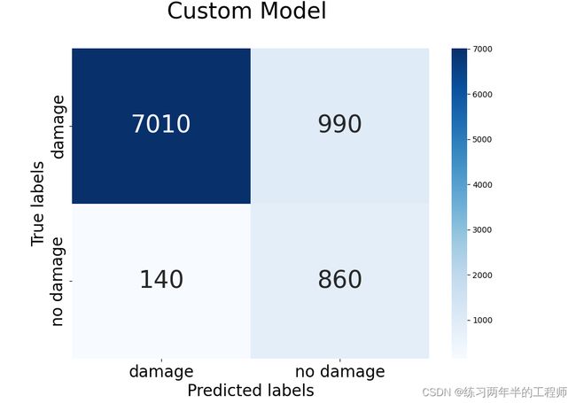
acc_rate = 100*accuracy_score(y_actual, y_predict)
print("The Accuracy rate for the model is: ", acc_rate)
print(confusion_matrix(y_actual, y_predict))

cm = confusion_matrix(y_actual, y_predict)
fig = plt.figure(figsize = (10,7)) # 创建一个图形对象 fig，用于绘制热力图
ax= plt.subplot() # 创建一个子图对象 ax，用于在图形中绘制内容
sns.heatmap(cm, cmap="Blues", annot=True, ax = ax, fmt='g', annot_kws={"size": 30}) # cm 包含了混淆矩阵的数据，cmap 指定了颜色图谱，annot=True 表示在图中显示数值，fmt='g' 表示使用一般数值格式，annot_kws={"size": 30} 指定了数值的字体大小

输出为：
The Accuracy rate for the model is: 87.44444444444444
[[7010 990]
[ 140 860]]

13. 将混淆矩阵图表保存为文件

ax.set_xlabel('Predicted labels',fontsize= 20) # 设置横轴标签和字体大小
ax.set_ylabel('True labels',fontsize= 20) # 设置纵轴标签和字体大小

ax.set_title('Custom Model \n',fontsize= 28)

ax.xaxis.set_ticklabels(['damage', 'no damage'],fontsize= 20) # 设置横轴刻度标签和字体大小
ax.yaxis.set_ticklabels(['damage', 'no damage'],fontsize= 20) # 设置纵轴刻度标签和字体大小
ax.yaxis.set_major_locator(ticker.IndexLocator(base=1, offset=0.5)) # 设置纵轴刻度主要定位器，以便正确显示刻度

fig.savefig("Result_Confusion_Matrix_Custom.png")