【编程实践】复杂网络的基本知识及实现

1 创建网络

1.1 创建一个图(Graph)

四种类型：无向图、有向图、多层无向图、多层有向图

// 共有四种类型
import networkx as nx
G = nx.Graph()
G = nx.DiGraph()
G = nx.MultiGraph()
G = nx.MultiDiGraph()

1.2 创建图的节点(Node)

任何类型都可以成为一个节点，一个数字 、一个字符、甚至一个带参数的函数

// 方法一
G.add_node(1)#节点是数字
G.add_node('CHINA')#节点是字符
def ff(a,b):
	c=(a+b)*(a-b)
	return c
G.add_node(ff(5,3))#节点是函数,会增加一个节点标签为16的节点
// 方法二:从一个列表中获取节点
G.add_nodes_from([10,20,30,40,50])
// 方法三：从一个列表中获取，但是列表中包含描述节点属性的字典
G.add_nodes_from([
	('CHINA',{"color":"blue"}),
	('USA',{"color":"blue"}),
	('UK',{"color":"blue"})
	])

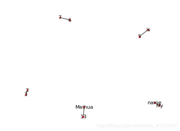
1.3 创建图的边(Edge)

//方法一
G.add_edge('My','name', weight=4.7 )
//方法二
G.add_edges_from([('is', '5'), ('6', '7')], color='red')
//方法三
G.add_edges_from([('Meihua', '13', {'color': 'blue'}), (2, 3, {'weight': 8})])

>>>print(G['My']['name']['weight']))
>>>4.7#可计算得出该条边的权重为4.7

1.4 其他方法

// 其他常用的网络操作方法
Graph.__init__([incoming_graph_data])
Graph.remove_node(n)
Graph.remove_node(nodes)
Graph.add_weighted_edges_from(ebunch_to_add)
Graph.remove_edge(u,v)
Graph.remove_edges_from(ebunch)
Graph.update([edges,nodes])
Graph.clear()
Graph.clear_edge()

1.5 网络数据集

Stanford大学大规模网络数据集：http://snap.stanford.edu/data/

2 网络指标-节点属性

2.1 度-Degree

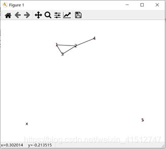
解释：这里的节点“5”为什么度值为2，是因为这里“5”这里是是一个起点和终点都为“5”的边，因为重合所以就没有边就没有绘制出来，但是边和度值却依旧存在。

// 计算每个节点的度
Nodes_list=[]#一个装有节点的列表
D=[]
for i in range(len(Nodes_list)):
	d=G.degree(Nodes_list[i])#临时变量
	D.append(d)#一个装有度的列表

2.2 度中心性-Degree Centrality

Degree Centrality，in case of weighted and directed network in a graph, an actor’s degree is defined by the number of another actors that directly connected to him as in-degree, vice versa out-degree. Node size that formed by actor depends on the metric. The most influence actor can be generated from the biggest value in-degree centrality . Where d[i] is the degree (number of adjacent edges) of node v[i].

// 计算度中心性，返回一个列表
nx.degree_centrality(G)

2.3 平均路径长度

// 计算网络的平均路径长度，返回一个数值
nx.average_shortest_path_length(G)

2.4 簇系数-Cluster

// 计算网络的簇系数，返回一个列表
clu=nx.clustering(G)

网络的簇系数：取值范围为[0,1]
相邻节点也相邻的数目/该节点所有边的数目，比如节点2的簇系数=1和3的形成的一条边/节点2所有相邻的边=1/3=0.333；单一一个节点的簇系数为零；
下图简易网络的簇系数计算结果为{1: 1.0, 2: 0.333, 3: 1.0, 4: 0, 5: 0, ‘x’: 0}

2.5 接近中心性-Closeness Centrality

紧密度（Closeness）可用来度量网络中的节点通过网络对其他节点施加影响的能力。节点的紧密度越大，表明该节点越居于网络的中心，在网络中越重要。
Clossness Centrality directly relates to the geodesic distance (or the cardinality of the shortest path) between two actors. It has a reflection of the whole connectivity in the network structure. Where d(i,j) defines the distance between two actors i and j, n is number of nodes/actor.

// 计算节点的接近中心性，返回一个列表
clo_cen=nx.closeness_centrality(G)

2.6 中介中心性-Betweenness Centrality

中介中心性（Betweenness Centrality）以经过某个节点的最短路径来刻画节点重要性的指标。该指标用于衡量个体社会地位。
Betweenness centrality depicts the position of an actor in between, so he can control other two actors, which do not have direct connectivity between them. This metric is important in global centrality measure, which investigates the strength of connectivity between the actors in the network. Where ,pjk is the number of geodesic paths between two actors j and k, and pjk(i) is the number of geo desic paths between j and k that contains actor i.

// 网络的介数中心性，返回一个列表
bet_cen=nx.betweenness_centrality(G)

2.7 特征向量-Eigenvector

特征向量（Eigenvector）一个节点的重要性既取决于邻居节点的数量，也取决于邻居节点的重要性。度指标把周围邻居视为同等重要， 这些邻居的重要性是不一样的，考虑到节点邻居的重要性对给节点的重要性有一定影响。如果邻居节点在网络上中很重要，则这个节点的重要性可能很高；如果邻居节点的重要性很低，即使邻居节点的邻居很多，则该节点不一定很重要。通常称这种情况为邻居节点的重要性反馈。特征向量指标是网络邻接矩阵对应的最大特征是的特征向量。

// 计算每一个节点的特征向量中心性，返回一个列表
eig_cen=nx.eigenvector_centrality_numpy(G)

指标名称	概念
点中心度	在某个点上，有多少线。某点单独的价值
接近中心度	该点与网络中其他点距离之和的倒数，越大说明越在中心，越能够很快到达其他节点。强调点在网络的价值，越大，越在中心。体现用户的价值
中介中心度	代表最短距离是否都经过该点，如果都经过说明这个点很重要，其中包括线的中心度。强调点在其他点之间调节能力，控制能力指数，中介调节效应。体现用户的控制力
特征向量中心度	根据相邻点的重要性来衡量该点的价值，首先计算邻接矩阵，然后计算邻接矩阵的特征向量。强调点在网络的价值，并且与接近中心度不同的在于，点价值是根据邻居节点来决定的。体现节点的潜在价值

2.6 小世界效应“Small world”

复杂网络的小世界效应是指尽管网络的规模很大(网络节点数目N很大)，但是两个节点之间的距离比我们想象的要小得多。也就是网络的平均路径长度L随网络的规模呈对数增长，即L～In N。大量的实证研究表明，真实网络几乎都具有小世界效应。最出名就是社会学中的“六度分形理论”。

2.7 无标度特性

无标度特性反映了复杂网络具有严重的异质性，其各节点之间的连接状况（度数）具有严重的不均匀分布性：网络中少数称之为Hub点的节点拥有极其多的连接，而大多数节点只有很少量的连接。